(updated 24th March 2023 to include a section on alteration of the rivers network to improve searchability (see Section 10 )
Overview
Maps and networks have always fascinated me, which is why I’m excited to explore and manipulate a dataset on waterways in this post. This dataset is both geospatialandtopological which makes it the basis for both a map and a network route-planner! In turn, this makes it very interesting to me, and complementary to the other opendata datasets I’ve already explored in this series:
The dataset I’m exploring here is the Open Rivers dataset for the UK published by the Ordnance Survey. The Ordnance Survey is an organisation steeped in history stemming back to 1745. It began life supporting military strategy, but has grown into Britain’s mapping agency. It has embraced opendata and publishes very good datasets (mainly geospatial) on all sorts of things. The OS open-river dataset will allow me to draw maps like the one shown below, and so much more.
I hope you find this post interesting and useful.
The OS Open Rivers dataset enhanced to highlight river networks
The geo-spatial and topological qualities of this dataset will help me navigate the rivers in a way akin to a route-planner, something I’ll explore in this post, and really hope to exploit in subsequent posts.
Aside: There is an entire ecosystem of GIS software out there to support drawing maps and geospatial analysis. Many are excellent and can be found by web-searches. In the FOSS1 world, QGIS is the GUI based GIS I use most. However… In this post I will be using R as it allows fully reproducible data processing and supports publication of the entire process in posts like this. I use a package called “sf” for geospatial processing, and subsequently a meta-package called “sfnetworks”2 throughout. When we’re dealing with geospatial data there are a wide range of packages that help load, manipulate and visualise geospatial and network datasets. See this resource from r-spatial.org, this and many other brilliant resources are signposted in the big book of R.
Step 0: Prepare some Libraries
First there’s the obligatory step of loading the libraries that I’ll be using throughout this post:
Code
library(tidyverse) # this blog uses the tidyverselibrary(lubridate) # I'm sure lubridate has been added to the tidyverse, old habits die hardlibrary(httr) # we will use this to collect data from the internetlibrary(sf) # I'm going to plot some maps. sf helps with any spatial stufflibrary(leaflet) # I like the interactivity of leaflet, but there are many other packages to plot maps.library(progress) # for feedback on progress during any long data downloadslibrary(htmltools) # I'll use this to customise some tables in the codelibrary(tidyjson) # the edivalent of tidyr for json objects (returned from URLs)
Step 1: Loading the OS rivers data
Collect the rivers data from Ordnance Survey
I’m accessing river data from here: OS Open Rivers - data.gov.uk3. The OS provide this dataset in a number of formats. I have collected the dataset in GeoPackage format4 from this URL and saved it before running the code in this post5.
Once downloaded6 We can have a quick look at the contents of the geo-database before loading it. We can see that the dataset has two layers (hydro_node and watercourse_link) …
Code
# note: I did try to automate this task based on# https://stackoverflow.com/questions/64850643/why-cant-i-get-st-read-to-open-a-shapefile-from-a-compressed-file-map-is-readsf::st_layers("C:/Users/leoki/DATA/OS/oprvrs_gpkg_gb/data/oprvrs_gb.gpkg")
Driver: GPKG
Available layers:
layer_name geometry_type features fields crs_name
1 HydroNode Point 194325 2 OSGB36 / British National Grid
2 WatercourseLink Line String 190069 9 OSGB36 / British National Grid
It requires only one line of code to load each layer. As each layer is loaded we get a summary of its geo-spatial attributes (like what’s the geometry type, the number of records, the Coordinate Reference Systems etc.).
Reading layer `WatercourseLink' from data source
`C:\Users\leoki\DATA\OS\oprvrs_gpkg_gb\data\oprvrs_gb.gpkg'
using driver `GPKG'
Simple feature collection with 190069 features and 9 fields
Geometry type: LINESTRING
Dimension: XYZ
Bounding box: xmin: 64429.59 ymin: 13274.99 xmax: 655208.5 ymax: 1216428
z_range: zmin: 0 zmax: 0
Projected CRS: OSGB36 / British National Grid
The summary tells us that:
Both layers have geometries and hence can be added to maps. The geometry of os_or_hydro_node is points and that of os_or_watercourse_link is lines. Points and Lines are two of the fundamental building blocks of geospatial analysis and are often complemented by the third type; polygons (such as the water company boundaries I loaded in part 2 of this series). I will load the water company boundaries again later in this post to compare against some things I’ll generate en-route within this blog.
os_or_hydro_node: The nodes are virtual way-points on the rivers. There are 194,325 nodes, each one has a unique identifier and some information on the nature of each section of the river (which we will soon see is only partially complete).
Code
os_or_hydro_node %>%# I dont need to convert to a tibble but it's faster if I doas_tibble() %>%count(hydroNodeCategory, sort = T)
os_or_watercourse_link: The links represent segments of the rivers themselves. There are 190,069 links, each one includes a range of information about the section of river. A sample of the links is shown below. Each of the 9 plots of the rivers in Great Britain is a field in the links dataset, only entries that are not blank are plotted on the maps. Notice that the watercourseNameAlternative is only sparsely populated. I will dig a bit deeper into the contents of each field in the next section.
Code
os_or_watercourse_link %>%# we dont need to plot all 190k lines# to get a n idea of the content# so I'll only plot 5ksample_n(5000) %>%plot()
Exploring the OS open-rivers data
It is good to spend time when first loading some data to get to know it. There are lots of packages out there that can help. This blog from littlemissdata contains a really good summary of some options. In this post I’ll just have a quick “skim” of the links to get to know the dataset a bit better.
The id and geom columns are unique (there are as many distinct values as there are rows in the dataframe). These are “high cardinality”. In this extreme case, the entries can be used as unique identifiers for each record.
the form column contains a categorical classification for each node (see below). These are “low cardinality” (there’s only a few alternatives). These kinds of fields are often categorical7.
# A tibble: 25,991 × 3
watercourseName watercourseNameAlternative n
<chr> <chr> <int>
1 <NA> <NA> 89690
2 River Avon <NA> 599
3 River Thames <NA> 326
4 River Stour <NA> 291
5 River Derwent <NA> 275
6 River Spey <NA> 275
7 River Dee <NA> 271
8 Afon Hafren River Severn 259
9 River Great Ouse <NA> 250
10 River Tweed <NA> 238
# … with 25,981 more rows
It is a little worrying that there are many links that have not been assigned either a name or an alternativeName. (shown as “<NA>” in the table shown above). I will have to explore some more to understand what’s going on here.
Diving deep into a single river (The Thames)
When exploring a new dataset it can help to focus on a specific aspect or use-case. It can be especially helpful if one can relate to some aspect of the data. For that reason, I’ll focus on the River Thames as I have lived close to this river all my life.
Code
# even though I know I'm going to looko at the river Thames I'll make it a variable# it's a good habbit.# also, I've explored other rivers before publishing and the use of a variable helped# as an exercise for the reader: what's odd about these two catchments: "yare", "waveney"target_river <-"river thames"
The plot below shows that the River Thames (as selected using the name attribute) has a number of discontinuities, for example the River looks to stop and start again inside the red box.
Code
bbox_thames <-tribble(~lat, ~lon, 51.4, 0.1,51.55,0.35) %>%st_as_sf(coords =c("lon", "lat"), crs =4326) %>%st_bbox() %>%st_as_sfc()os_or_watercourse_link %>%filter(str_detect(str_to_lower(watercourseName), target_river)|str_detect(str_to_lower(watercourseNameAlternative), target_river)) %>%ggplot() +geom_sf(aes(colour = form)) +geom_sf(data = bbox_thames,colour ="red", alpha =0.01, linewidth =1) +labs(title =paste0("OS water Courses filttered to thgose named: ", str_to_title(target_river)),subtitle =paste0("Part of the river (boxed) is not labelled as: '", str_to_title(target_river), "'"))
This kind of exploratory Data Analysis (EDA) is probably best done in GIS software (e.g. QGIS), but this simple map allows exploration of names and alternativeNames of all water courses in that region. Hovering over the blue lines will show the parts of the Thames that do not appear in the previous plot are part of the dataset but have no names assigned whatsoever.
Not to worry! Later in this post we will see there are ways to handle these gaps and find our way from source to outlet of the River Thames regardless (assuming some other aspects of the dataset are good enough). To do this I will be exploring two other properties of the datasets
The nodes have that hydroNodeCategory classification (source, outlet, junction etc.)
The links have a fromNode and a ToNode which allow them to be connected. I’ll be using the connectivity of the river sections to allow me to navigate along rivers like the Thames regardless of the sections being fully labelled.
Step 2: A Digital Twin of the river network?
There’s a lot of hype about digital twins at the moment, and I want to say that I’m creating one here. But before I do…
Just what is a digital twin?
One definition is that digital twins are digital representations of an object or system that accurately reflects aspects of the system’s behaviour. So what’s the difference between a digital twin and what was once called a simulation or a model? A key characteristic is that a digital twin is associated (twinned) with an object that actually exists (a model / simulation can be of something that does not exist). It might be useful here to compare a flight-simulator against the internal models of a fly-by-wire aircraft. Both need to digitally represent the flight characteristics of an aircraft, but only one is linked to a real aircraft. Because digital twins always have a real twin, they have an extra requirement to represent some aspect of that object well enough to be used to generate insight about the real version. If the real object can have different states, then the digital twin will need to reflect those states, which in turn often requires information on the real twin to be gathered from sensors.
Am I really creating a digital twin here?
My overall goal for this series of posts is to join the river data explored in this post (such as connectivity, length and paths taken) with the water that is in the river at any given time (such as level and flow data shared by the EA as explored in post 2) and what’s being discharged into the rivers (such as storm surge data, from post 1).
For the sake of drama I’ll say yes, eventually I’ll have created a digital twin of the river network. It will be limited in that it will know nothing about things like hydraulics or open-channel flows. It wont even know the gradient of the rivers nor their width or other pertinent details.
For now though, no I wont call this a digital twin, I’ll just call this a map of the UK rivers. However, I am heading in the right direction…. The next section will turn the map of the UK rivers into something closer to a model of UK rivers when I begin to consider how all the individual sections of rivers are joined together to create river networks.
Step 3: Rivers as Maps and Networks
As described earlier, the OS open rivers dataset includes information on both the individual sections of rivers and how they connect together. This means that I can build a network (sometimes called a graph) from the river data… With this I can do more than just know where the rivers are… I can know where they are going, where they come from, and how they are interlinked into systems.
I have used a fantastic R package called {sfnetworks} in this post. In turn, it uses {sf} for geospatial manipulation (for example; linking to other spatial datasets) and {igraph} for network analysis (such as splitting the river network up into river systems or tracing along sections of rivers between points of interest).
First I create sfnetwork object which has all these amazing capabilities:
Code
# #| we're going up a gear... use sfnetworks to do both#| geospatial analysis (sf for geospatial manipulation)#| like slipping and linking other spatial datasets)#| and network analysis (igraph for network type analysis)#| like splitting the river network up into river systems#| or tracing along sections of rivers from point to pointlibrary(sfnetworks)# create a sf network for the whole of the UK ----# (takes a few seconds on my laptoi)sfnet_rivers <-as_sfnetwork(os_or_watercourse_link)#| note: the package can create networks from the nodes and links.#| like this: (IF(F) so it DOES NOT RUN)if(F) {# do not run! while this is how the documetation says to do it# it gobbles up all my laptp memory sfnet_rivers <-sfnetwork(nodes = os_or_hydro_node,edges = os_or_watercourse_link %>%rename(from = startNode, to = endNode),node_key ="id")}#| Including the nodes and the links will embue the sfnetwork#| with attributes of both the nodes and the links#| This is something 8 really want..#| HOWEVER, for some reason this chews up all the memory#| on my laptop before crashing.
Then I make sure that all the attributes of the OS datasets are carried over (I use SQL-like joins but there are a surely many ways to implement this step)
Code
#| ...then... adding some info back onto the nodes by:#| get the original IDs for the nodes from the link start/ends#| so that we can then link in the information from the os_or_hydro_node sfnet_rivers <- sfnet_rivers %>%# hereactivate(links) %>%# look up the hydroNodeCategory of the startNodeleft_join(os_or_hydro_node %>%as_tibble() %>%as_tibble() %>%select(-geom) %>%rename(startNode = id, start_cat = hydroNodeCategory)) %>%# look up the hydroNodeCategory of the endNodeleft_join(os_or_hydro_node %>%as_tibble() %>%as_tibble() %>%select(-geom) %>%rename(endNode = id, end_cat = hydroNodeCategory)) %>%# hereactivate(nodes) %>%# reunite the nodes with the startNode & endNode ids# look up the startNode of links connected FROM itmutate(id =row_number()) %>%left_join(sfnet_rivers %>%activate(links) %>%as_tibble() %>%transmute(id = from, startNode) %>%# FROM# transmute(id = from, startNode, start_watercourse = coalesce(watercourseName, watercourseNameAlternative)) %>% # FROMas_tibble() %>%select(-geom) %>%distinct() ) %>%# look up the end of links connected TO itleft_join(sfnet_rivers %>%activate(links) %>%as_tibble() %>%transmute(id = to, endNode) %>%# TO# transmute(id = to, endNode, end_watercourse = coalesce(watercourseName, watercourseNameAlternative)) %>% # TOas_tibble() %>%select(-geom) %>%distinct() ) %>%# both TO & FROM should hold the same chr ID# sometimes one or the other will be blank (at the ends of the network)# so lets collapse the IDs from either by coalescingmutate(node_id =coalesce(startNode, endNode)) %>%rename(startNodeFromLinks = startNode, endNodeFromLinks = endNode) %>%left_join(os_or_hydro_node %>%as_tibble() %>%as_tibble() %>%select(-geom),by =c("node_id"="id"))
I can delete the original datasets as they’re both absorbed into the new {sfnetworks} object I’ve called sfnet_rivers.
Route finding: tracing a river from source(s) to outlet
The OS data is now in a form that is both a map and a network. I can do some really useful next-level things like finding the shortest path between the objects9. Let’s try tracing the River Thames along its entire path. First I have to define where I want to start and end. In this example I want to find a route between the westernmost point on the River Thames to its outlet into the North Sea.
Code
#| note: I'm going to find points on rivers more than once#| in this post, so in the spirit of DRY....#| I'll encapsulate the logic in a function#| INPUTS:#| sfnetwork - the network to be searched#| river_name - a river to filter on (case insensitive)#| node_category - and hydroNodeCategory (case insensitive)#| RETURNS:#| a dataframe containing the nodes matching the filtersfind_all_nodes <-function(sf_net, river_name, node_category){if(!hasArg(river_name)) {warning("find_all_nodes: river_name not defined (returning NULL)")return(NULL) }if(!hasArg(node_category)) {warning("find_all_nodes: node_category not defined (returning NULL)")return(NULL) }# Step 1: filter nodes of the required type river_nodes <- sf_net %>%activate(nodes) %>%mutate(id =row_number()) %>%as_tibble() %>%as_tibble() %>%filter(hydroNodeCategory ==str_to_lower(node_category))# step 2: filter rivers to the target river_nameif(str_to_lower(node_category) =="source") { river_nodes <- river_nodes %>%inner_join( sf_net %>%activate(links) %>%as_tibble() %>%as_tibble() %>%filter(str_detect(str_to_lower(watercourseName),str_to_lower(river_name))|str_detect(str_to_lower(watercourseNameAlternative),str_to_lower(river_name))) %>%select(node_id = startNode) ) } else { river_nodes <- river_nodes %>%inner_join( sf_net %>%activate(links) %>%as_tibble() %>%as_tibble() %>%filter(str_detect(str_to_lower(watercourseName),str_to_lower(river_name))|str_detect(str_to_lower(watercourseNameAlternative),str_to_lower(river_name))) %>%select(node_id = endNode) )return(river_nodes) }} # end of find_all_nodes()# now we can get the outlet of the River Thames:river_outlet_node <-find_all_nodes(sf_net = sfnet_rivers,river_name ="River Thames",node_category ="outlet") %>%# thre is only one outlet for the Thames,# but if there were more, we might wantr to filter to# only include the eastern-most node:st_as_sf(crs =st_crs(27700)) %>%mutate(lon = sf::st_coordinates(.)[,1],lat = sf::st_coordinates(.)[,2]) %>%#| then arrange the rows east -> west#| (longitude is smallest in the west so this is descending)arrange(desc(lon)) %>%# select the (single) easternmost nodeslice(1)# rivers in this dataset have a lot of sourceswesternmost_target_node <-find_all_nodes(sf_net = sfnet_rivers,river_name ="River Thames",node_category ="source") %>%st_as_sf(crs =st_crs(27700)) %>%mutate(lon = sf::st_coordinates(.)[,1],lat = sf::st_coordinates(.)[,2]) %>%#| then arrange the rows west -> east#| (longitude is smallest in the west)#| and somewhere later on, I'll pick the first (most westerly)#| source.#| I could have included all sources then in the route-planning#| and then chosen the one that had the longest patharrange(lon) %>%# select the (single) westernmost nodeslice(1)
Then we can trace from the start to the end, picking up all links inbetween. The route we’re about to generate is similar to that taken by the three men and a dog in Jerome K. Jerome’s book Three Men In a Boat)
Code
# this just gets the path to the outletpaths_downstream_target <-st_network_paths(sfnet_rivers,from = westernmost_target_node$id,to = river_outlet_node$id,weights ="length") %>%mutate(n_nodes =lengths(node_paths))# lets have a look at the path...sfnet_rivers %>%activate("nodes") %>%#| probably should use sfnetwork spatial morphers#| https://luukvdmeer.github.io/sfnetworks/articles/sfn05_morphers.htmlslice(unique(unlist(paths_downstream_target$node_paths))) %>%activate(links) %>%st_transform(crs =st_crs(4326)) %>%mutate(geom =st_make_valid(geom)) %>%st_as_sf() %>%# as_tibble() %>%# mutate(namesThames = coalesce(namesThames, "No")) %>%leaflet() %>%addTiles(group ="OSM (default)") %>%addProviderTiles(providers$Stamen.Terrain, group ="Terrain") %>%addPolylines(label =~paste0(watercourseName, ' - ', watercourseNameAlternative) ) %>%addLayersControl(baseGroups =c("OSM (default)", "Terrain"),options =layersControlOptions(collapsed =FALSE) )
Aside: Remember how much trouble there was finding all the parts of the River Thames based on the watercourseName attribute because some of the river segments had not been labelled? The route-finding way has collected all the parts of the river between the source(s) and the outlet. If one wished, one could then apply some (carefully validated) domain rules to assert that all the links between should be called “River Thames” and cleans the watercourseName to be more complete, infilling those blanks with something more sensible. (I’m not going to do this here).
Remember rivers have a sense of direction…
The river network is a “directed graph”, in the sense that water flows from here to there. The sfnet_rivers object has all this information on direction and connectivity. This means that the rivers are like one-way-streets in a route-planner. By default the shortest paths algorithm will only go in the direction from->to. It’s easy to ask it to look the other way (e.g. to find all tributaries of a river) but you have to explicitly ask it to search upstream.
Tracing upstream towards some points of interest
In the example below I will find all routes upstream from the outlet of the Thames to any source of either the Thames or the River Kennet. The River Kennet is a tributary of the River Thames, joining at Reading. So first lets find the source(s) of both rivers.
The function returned a total of 78 places marked as “source” on the Thames and the Kennet. I would have expected only one source per river, so have explored this a little. Having looked into this, it seems the OS open-rivers dataset classifies “source” as the part of a river that rejoins at the point where it runs through a lock and around a weir.
Let’s plot all the shortest paths between all the sources (on the Kennet and Thames) and the outlet of the Thames.
Code
# this just gets the path to the outletpaths_upstream_to_sources <-st_network_paths( sfnet_rivers,from = river_outlet_node$id,to =unique(c(source_thames_nodes$id, source_kennet_nodes$id)),weights ="length",mode ="in") %>%#c("out", "all", "in")mutate(n_nodes =lengths(node_paths))
Warning in shortest_paths(x, from, to, weights = weights, output = "both", : At
core/paths/dijkstra.c:442 : Couldn't reach some vertices.
Code
# lets have a look at the path...sfnet_rivers %>%activate("nodes") %>%# slice(unlist(kennet_paths$vpath)) %>%slice(unique(unlist(paths_upstream_to_sources$node_paths))) %>%activate(links) %>%st_transform(crs =st_crs(4326)) %>%mutate(geom =st_make_valid(geom)) %>%st_as_sf() %>%# as_tibble() %>%# mutate(namesThames = coalesce(namesThames, "No")) %>%leaflet() %>%addTiles(group ="OSM (default)") %>%addProviderTiles(providers$Stamen.Terrain, group ="Terrain") %>%addPolylines(label =~paste0(watercourseName, ' - ', watercourseNameAlternative) ) %>%addLayersControl(baseGroups =c("OSM (default)", "Terrain"),options =layersControlOptions(collapsed =FALSE) )
Plotting rivers as a tree (dendrogram)
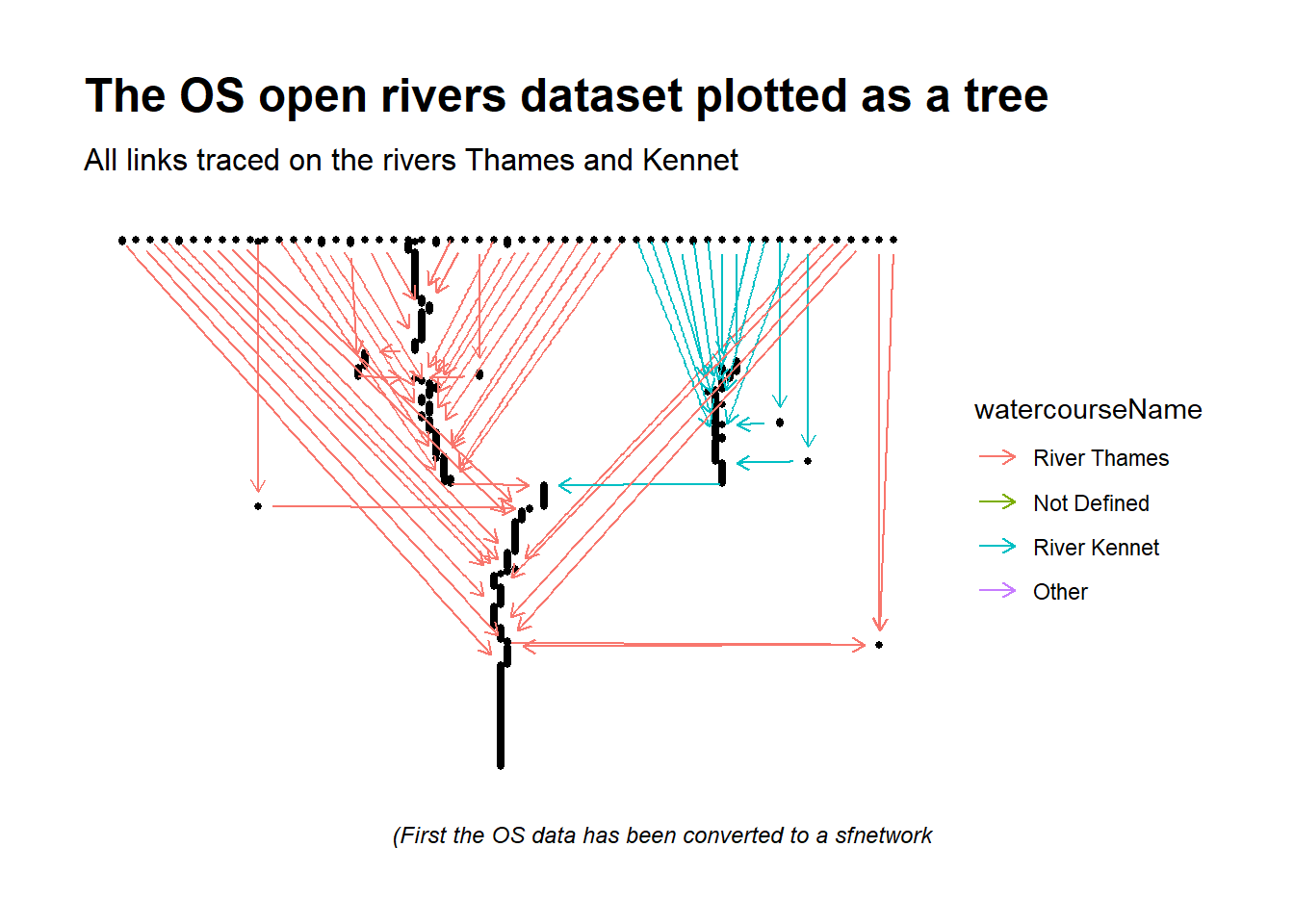
Rivers and their tributaries resemble trees. While trees branch out, rivers connect together. I’ve generated a plot (below) simply to highlight how, what may once have appeared to be “just” a geospatial set of data that could be plotted on a map, is now very-much a network of interconnected elements. The plot below has limited the full rivers network to highlight only the branching nature of the sections of river on the Thames and the Kennet that feed into the sea at the mouth of the Thames.
Code
library(ggraph)library(igraph)thames_kennet_subgraph <- sfnet_rivers %>%activate("nodes") %>%slice(unique(unlist(paths_upstream_to_sources$node_paths))) %>%activate(links) %>%# if we wanted to simplifyto remove nodes that have only one incoming and one outgoing edge. # https://luukvdmeer.github.io/sfnetworks/articles/sfn02_preprocess_clean.html#smooth-pseudo-nodes# tidygraph::convert(to_spatial_smooth) %>%mutate(watercourseName =coalesce(watercourseName, "Not Defined")) %>%mutate(watercourseName =as_factor(watercourseName)) %>%mutate(watercourseName =fct_lump_n(watercourseName, 3)) %>%as.igraph() thames_kennet_subgraph %>%ggraph() +# ggraph(layout = "dendrogram") +geom_node_point(size =1) +geom_edge_link(aes(colour = watercourseName), arrow =arrow(length =unit(2, 'mm'), ends ="last"),end_cap =circle(2, 'mm'),start_cap =circle(2, 'mm')) +theme_graph() +labs(title ="The OS open rivers dataset plotted as a tree",subtitle ="All links traced on the rivers Thames and Kennet",caption ="(First the OS data has been converted to a sfnetwork")
Because the OS open-rivers dataset is now a graph, we can run graph-related statistics such as centrality and betweenness. This might feel academic, but such statistics may come in handy when characterising river networks that are, for example, more or less likely to suffer when polluted.
Step 5: Augmenting with ‘systems of rivers’
The OS open-rivers dataset is both a map and a network. It is possible to do some very useful processing and generate some beautiful summaries.
For example, imagine we wanted to subdivide the whole of the UK into river ‘systems’. Where each system is a set of rivers that are connected somehow. This would be easy to implement if we had a big map of all the rivers and a box of colouring pens… we could create the systems by printing out a black and white map of all the rivers, and then:
Repeat the following:
take a new colouring pen from the box.
place the pen on a river on the map that hasn’t yet been coloured.
trace all the sections of all the rivers that can be reached without taking the pen off of the paper.
put that pen to one side
Until all rivers have been individually coloured.
Once complete, we would have defined all sub-networks of the main OS open-rivers dataset. In graph-theory what we have done is to define the components (sub-graphs) of the river network. This is something that can be implemented in one line of code with the help of the {igraph} package.
Code
# Step 1: calculate the components# mark each of the sub-graphs with a unique ID#| this ID is arbitrary but each river network has it's own IDrg <- igraph::components(sfnet_rivers)# Step 2: add the groups to the nodessfnet_rivers_grouped <- sfnet_rivers %>%# push the river group onto the nodesactivate("nodes") %>%mutate(rg =as_factor(rg$membership)) %>%group_by(rg) %>%mutate(n_nodes =n()) %>%ungroup()# Step 3: add the groups (of the end_node) to the linkssfnet_rivers_grouped <- sfnet_rivers_grouped %>%activate(links) %>%left_join( sfnet_rivers_grouped %>%activate(nodes) %>%as_tibble() %>%as_tibble() %>%transmute(endNode = node_id, rg, n_nodes) )# I dont need sfnet_rivers now. if I deleted it here# it would save me from accidentally rewfereing to it laterif(F) {rm(list ="sfnet_rivers")}
Deriving boundaries from systems of rivers
Let’s explore what has been generated by filtering the whole of the UK to the river system that contains the River Thames.
Aside: The water company boundaries are loaded here (this is the same code as was used in part 2 to trim the EA stations to the Thames Water operational region):
Code
#| Stack exchange once again makes it easy to make reproducible code#| https://stackoverflow.com/questions/64850643/why-cant-i-get-st-read-to-open-a-shapefile-from-a-compressed-file-map-is-readread_shape_URL <-function(URL){ cur_tempfile <-tempfile()download.file(url = URL, destfile = cur_tempfile) out_directory <-tempfile()unzip(cur_tempfile, exdir = out_directory) sf::read_sf(dsn = out_directory) #read_sf also works here st_read}wc_bundaries_sf <-read_shape_URL("https://data.parliament.uk/resources/constituencystatistics/water/SewerageServicesAreas_incNAVsv1_4.zip") %>%rename(geom = geometry) %>%# we don't need the full resolution here, save a few Mb# by simplifying to a tolerance of 10 meters because we're in CRS 27700st_simplify(dTolerance =10)
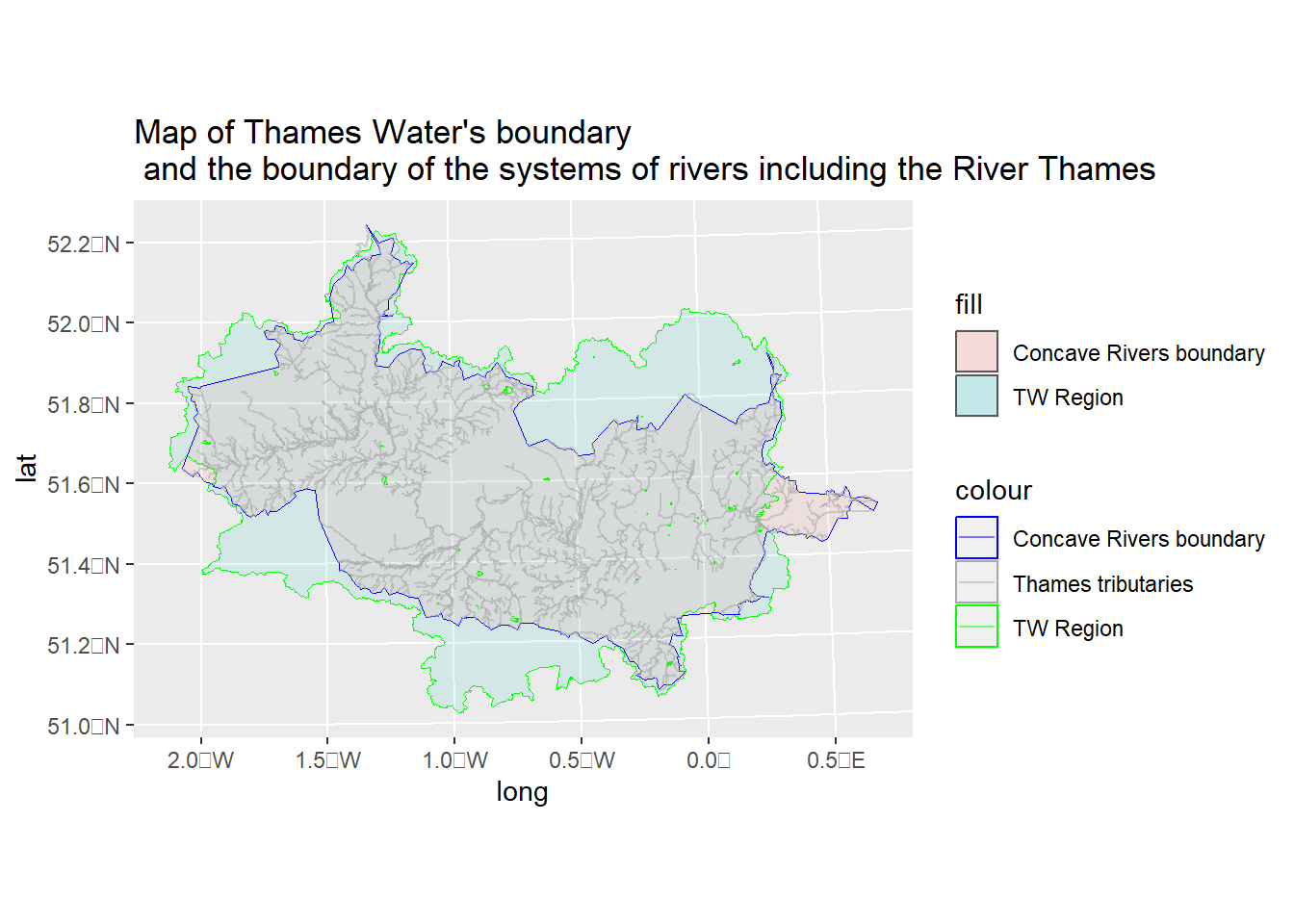
Now let’s compare the operational boundary of Thames Water with another boundary that has been solely defined by the perimeter of the system of rivers running into the sea at the mouth of the River Thames.
Code
# step 1: See which RG the river_outlet_node is part of...# (we created this my selecting the outlet of the Thames)this_rg <- sfnet_rivers_grouped %>%activate("nodes") %>%filter(node_id == river_outlet_node$node_id) %>%as_tibble() %>%select(rg) %>%as_tibble() %>%select(-geom) %>%head(1) %>%as.integer()# Step 2: Extract all the rivers that are part of# the river system that includes th river Thames sfnet_rivers_thames_basin <- sfnet_rivers_grouped %>%activate(links) %>%filter(rg == this_rg) %>%activate(nodes) %>%filter(!tidygraph::node_is_isolated()) %>%# the row number is out of date now (maybe drop entirely?)# it needs refreshing (or ignoring entirely!)mutate(id =row_number())# Step 3: Create a concave boundary for these riversconcave_rivers_boundary_sf <- sfnet_rivers_thames_basin %>%activate(nodes) %>%st_as_sf() %>%summarise() %>% concaveman::concaveman() %>%st_zm()#Step 4: plot them all on top of eachother#| https://community.rstudio.com/t/adding-manual-legend-to-ggplot2/41651/3#| to label the layerscolors <-c("Thames tributaries"="darkgrey","TW Region"="green","Concave Rivers boundary"="blue")ggplot() +geom_sf(data = wc_bundaries_sf %>%filter(COMPANY =="Thames Water"), aes(colour ="TW Region", fill ="TW Region"), alpha =0.1) +geom_sf(data = concave_rivers_boundary_sf, aes(colour ="Concave Rivers boundary", fill ="Concave Rivers boundary"), alpha =0.1) +geom_sf(data = sfnet_rivers_thames_basin %>%activate(links) %>%st_as_sf(), aes(colour ="Thames tributaries"), alpha =0.5) +labs(title ="Map of Thames Water's boundary\n and the boundary of the systems of rivers including the River Thames",x ="long",y ="lat") +scale_color_manual(values = colors)
The two areas look very similar but the Thames Water region is larger than that defined by the system of rivers. I’ve explored the area on the north-east of the disjoin between the Thames Water boundary and the concave boundary of the system of rivers including the River Thames. The reason for the north-east disparity is because there are short sections of the River Lea (alt name River Lee) that are not connected in the OS Open Rivers dataset (zoom right in to the red square in the map below to see the place where the rivers are disconnected). This disjoin may be deliberate, or it maybe an error in the dataset. If I were to chose the latter then I could do fixing-up of the OS dataset to join links that are (say) within some tolerance (I’ve added detail of such steps in the epilogue of this post entitled “joining the dots” @epilogue-augmentation ).
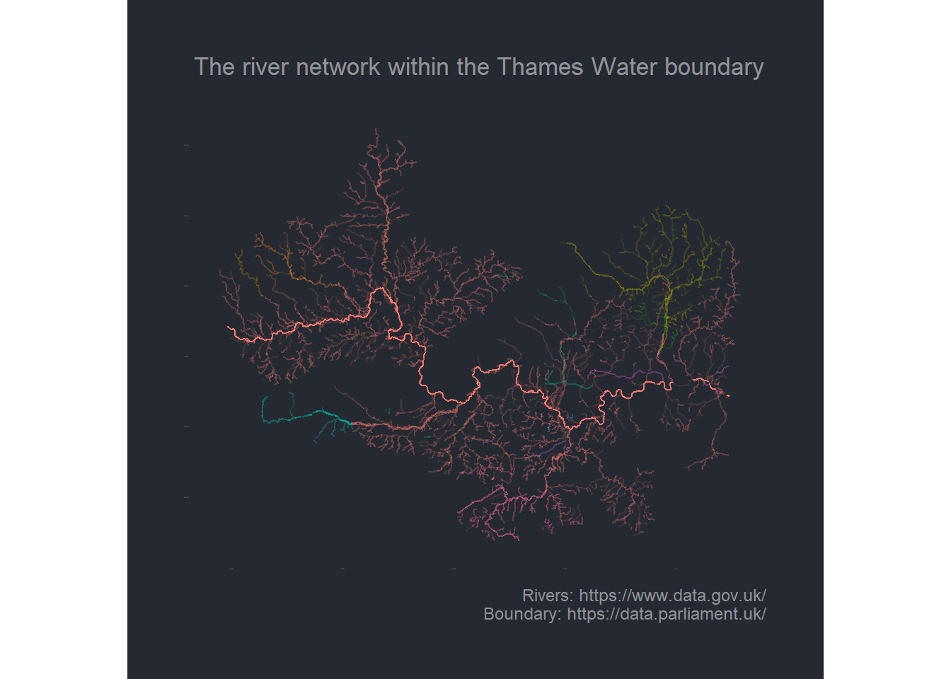
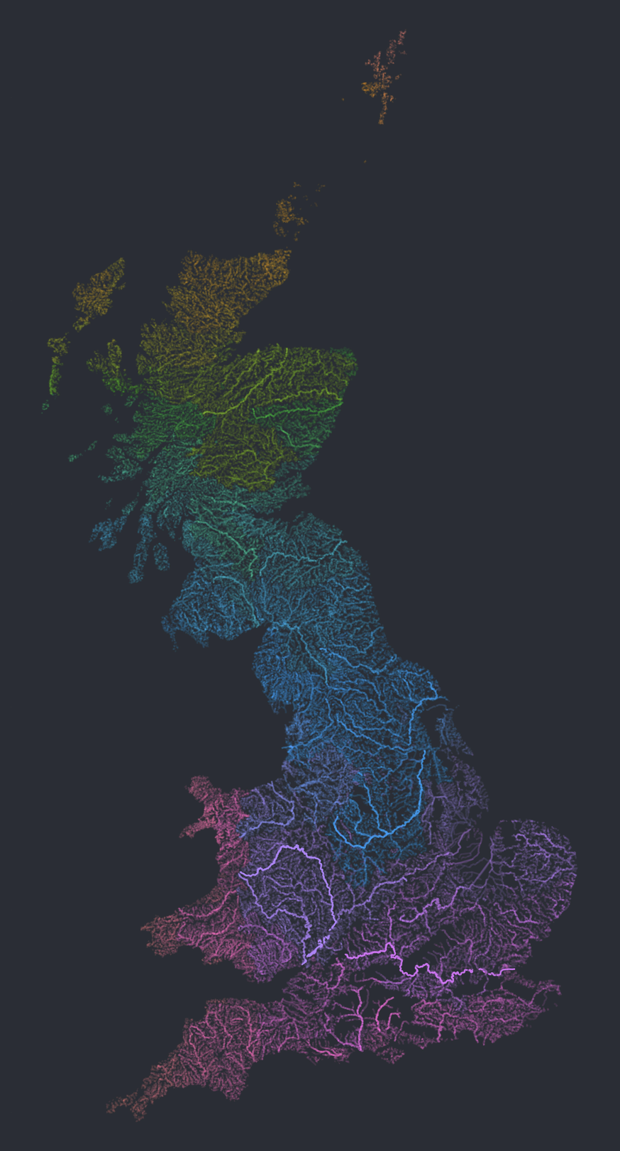
The logic outlined above to hand-draw the map of systems of rivers is precisely the logic I used when generating the colourful map at the very top of this post.
Each river system is plotted in it’s own colour. For aesthetic purposes, I have also made the lines more pronounced if the rivers are long, and less pronounced if the rivers are short.
The code which generated this plot is in the following section. The code below first cookie-cuts (filters) the whole of the UK so as to only include river systems that fall within the borders of the Thames Water operational area.
Code
# this code was used to generate and save the image.# in this blog I'm just loading the resultant image.# Note: I'm using ggplot to render the map however, # the ggplot rendering takes a long time.# there are faster ways but I;ve not included them here# as they're somewhat off-topic# draw the map tw_p <- sfnet_rivers_grouped %>%activate(links) %>%st_as_sf() %>%# limit to those river in the Thames boundariesst_filter(wc_bundaries_sf %>%filter(str_detect(COMPANY, "Thames")) %>%st_simplify(dTolerance =100)) %>%# calculate the length of entire river (as I want to emphasis *all* links on longer rivers)group_by(watercourseName) %>%mutate(river_length =sum(length)) %>%ungroup() %>%mutate(all_length =sum(length)) %>%mutate(norm_length = river_length / all_length) %>%mutate(norm_length =ifelse(is.na(watercourseName), 0.01, norm_length)) %>%select(watercourseName, rg, length, river_length, norm_length, all_length) %>%ggplot() +geom_sf(aes(colour = rg, alpha = norm_length)) + hrbrthemes::theme_ft_rc(grid = F,axis_text_size = F) +theme(legend.position ="none") +labs(# title = "Thames Water",subtitle = glue::glue("The river network within the Thames Water boundary"),# x = "", y = "",caption ="Rivers: https://www.data.gov.uk/\nBoundary: https://data.parliament.uk/" ) # render using ggplot to the screen (ok for TW, but slow for UK)tw_p
Until I generated these plots, I’d never really seen the rivers of the UK in quite this way. There’s something very aesthetically pleasing about how they branch. I have found it really interesting that there are parts of the UK that have virtually no surface rivers whatsoever.
Data checkpoint
It feels like we’ve done a lot to augment the original OS open-rivers datasets, so perhaps it’s a good time to save this augmented dataset as a new gpkg with the extra information on the river groups. It might be that this was all we wanted to use R for and
The rest of the analysis would be done inside QGIS.
The augmented dataset is of value to other analysis and the checkpoint is a great place from which to share it.
Code
# heres a function I have written to sage a sfnetwork# into a geopackage so it can be loaded into something like QGIS# remember: This might be a single object, but it holds# two layers# nodes (points)# links (lines)# each with their own set of attributessave_sf_network_as_geopkg <-function(this_sfnet, target_gpkg) {message(paste0("Exporting sf_network links to: ", target_gpkg)) this_sfnet %>%activate(links) %>%st_as_sf() %>%st_write(dsn = target_gpkg, layer="links", append=FALSE)message(paste0("Exporting sf_network nodes to: ", target_gpkg)) this_sfnet %>%activate(nodes) %>%st_as_sf() %>%st_write(dsn = target_gpkg, layer="nodes", append=FALSE)message("done")}# example of how to call the functionif(F) { sfnet_rivers_grouped %>%save_sf_network_as_geopkg("C:/Users/leoki/DATA/LAK/os_river.gpkg")}
Epilogue: joining some dots
This section has been added about a month after the rest of this post was published. It focusses on the issues mentioned in Section 9.1 whereby parts of the river network appear to be disconnected (due to weirs or locks etc). When I originally explored this, I concluded that I would just note this observation, however a deeper-dive has shown that some of these “missing links” could legitimately be restored and significantly improve the search capabilities I explored in Section 8.1 and deployed in this online app.
There are lots of algorithms that one could imagine to join dots between parts of this river-network dataset. After some exploration, I’ve written a function called get_missing_links() that searches from “outlets” for nearby “sources”. The function has some parameters that allow me to control how far it will search, and whether the names of the river sources and outlets must match.
The function implements a form of Occam’s razor (the simpler explanation is more favourable), and follows the logic:
“It is easier to imagine a”missing link” to explain why the end of one river is very near the start of another, than to think of a legitimate condition where one river stops and another starts nearby (especially if both rivers have the same name)“.
The code is shown in the code section below.
Code
get_missing_links <-function(net =NULL, from_category ="source", to_category ="outlet", bridging_dist =100, match_name = T) {#| I'm going to search#| from *all* nodes of type "from_category" (outlets)#| to *all nodes of type "to_category" (sources)#| that are close enough (defined by bridging_distance)#| I have an optional extra requirement that#| the names of the from & to nodes match#| In english...#| "IF there's a river source *really close* to a river source#| THEN it's possible that they should be connected#| (occam's razor: it's easier to explain why the end of one river is near the start of another through a "missing link" that to think of a legitimate condition where one river stops and another river starts nearby)#| ESPECIALLY IF they're both the SAME RIVER NAME all_start_nodes <- sfnet_rivers_grouped %>%activate(nodes) %>%st_as_sf() %>%filter(hydroNodeCategory %in% from_category) %>%left_join( sfnet_rivers_grouped %>%activate(links) %>%as_tibble() %>%as_tibble() %>%select(id = from, watercourseName) ) all_end_nodes <- sfnet_rivers_grouped %>%activate(nodes) %>%st_as_sf() %>%filter(hydroNodeCategory %in% to_category) %>%left_join( sfnet_rivers_grouped %>%activate(links) %>%as_tibble() %>%as_tibble() %>%select(id = to, watercourseName) )# *all* links between outlets and sources# we'll filter out anything that too far apart later from_to <-st_join(all_end_nodes, all_start_nodes,join = st_nearest_feature) %>%as_tibble() %>%rename(geom_start = geom) %>%rename_at(vars(contains(".x")), function(x) { str_replace_all(x, ".x", "_start") }) %>%rename_at(vars(contains(".y")), function(x) { str_replace_all(x, ".y", "_end") })if(match_name) { from_to <- from_to %>%filter(watercourseName_start == watercourseName_end) }# https://stackoverflow.com/questions/49853696/distances-of-points-between-rows-with-sf pos_link_start_ends <- from_to %>%transmute(watercourseName =coalesce(watercourseName_start, watercourseName_end), id_start, geom_start, id_end) %>%left_join(all_start_nodes %>%as_tibble() %>%transmute(id_end = id, geom_end = geom)) %>%mutate(length =st_distance(geom_start, geom_end, by_element = T), ) %>%filter(length < units::set_units(bridging_dist, m)) %>%arrange(desc(length)) new_links <- pos_link_start_ends %>%as_tibble() %>%mutate(length =as.numeric(length)) %>%mutate(id =row_number(), .before =1) %>%pivot_longer(cols =c(geom_start, geom_end), names_to ="pos", values_to ="geom") %>%st_as_sf() %>%group_by(id, id_start, id_end, watercourseName, length) %>%summarise(do_union =FALSE) %>%ungroup() %>%st_cast("LINESTRING") %>%transmute(from = id_start,to = id_end,length = length,form ="",watercourseName = watercourseName,start_cat ="",end_cat ="",rg =as_factor(1),n_nodes =as.integer(2) ) %>%st_as_sf() %>%# st_make_valid(geom) %>%select( from, to, length, form, watercourseName, geom, start_cat, end_cat, rg, n_nodes ) %>%mutate(geom =st_make_valid(geom))return(new_links)}
I’ve found that the restriction on matching names misses some of the connections I would like to create, and 75 metres appears to be a reasonable search distance, small enough to not add links between the sources of one river to an outlet of another while being large enough to span most questionable gaps in the OS river data.
As is often the case in data cleansing, it was much easier to write the code that than it was to decide on the parameters that defined which data the code worked on. All of this required a lot of eye-balling. I used QGIS for some aspects but found that a little code to present the extra links sped-up the task of investigating potential missing links.
An example of the output of the exploratory diagnostic plot is shown below. the missing links are highlighted. The river network near the missing links is also loaded for context. I’ve added a simple hyperlink to a pop-up on each (green shaded) area. The hyperlink opens googlemaps centred on the location in question. googlemaps is a great resource to better understand what the ‘real-world’ looks like.
The code below creates the missing links
Code
# transform the network into lat-long, we're going to be usingf leaflet a lot heresfnet_rivers_grouped <- sfnet_rivers_grouped %>%st_transform(crs =st_crs(4326)) %>%# the next step is important# it collapses the geom into *just* eastinga and northing# feature geometries can be 3-dimentional i.e.include height (as Z / M)# Drop Z and/or M dimensions from feature geometriesst_zm() bridging_dist <-75#| 1) get potential missing linksmissing_links <-get_missing_links(sfnet_rivers_grouped,from ="source",to ="outlet",bridging_dist = bridging_dist,match_name = F)# 2) i'm going to explore the geography and network around these links# so I'll also create a polygon around each missing link (by buffering it)# this will be used both to plot and highlight AND to cookie-cut other datasetsbboxes_name_not_matched <- missing_links %>%st_buffer(dist = units::set_units(bridging_dist, m))
and these can be visualised as follows:
Code
# first, here are some useful function I've written to help explore...makeHTML <-function(htmlText){attr(htmlText, "html") <-TRUEclass(htmlText) <-c("html", "character") htmlText}buildGoogleMapsURLFromLatLong <-function(myLati, myLongi) { result <-paste0('<br>','<a href="https://www.google.co.uk/maps/@', gsub(" ", "", format(round(myLati, 8), nsmall =8)),",", gsub(" ", "", format(round(myLongi, 8), nsmall =8)), ',19z" .external target="_blank" rel = "noopener noreferrer nofollow" >','Show in Googlemaps</a>')}buildGoogleMapsURLFromStGeom <-function(thisGeom) { xy <-st_coordinates(thisGeom) theRes <-buildGoogleMapsURLFromLatLong(xy[,2], xy[,1])}# now lets explore where those potential missing links are to be found:leaflet() %>%addTiles(group ="OSM (default)") %>%# a sausage around the POIaddPolygons(data = bboxes_name_not_matched,popup =~makeHTML(paste0("Nearly outlet & source: ", format(round(length, 2), nsmall =2), '<br>',buildGoogleMapsURLFromStGeom(st_centroid(geom)))),color ="green",label =~paste0("Nearly outlet & source: ", format(round(length, 2), nsmall =2))) %>%# the nearby networkaddPolylines(data = sfnet_rivers_grouped %>%activate(links) %>%filter(!tidygraph::edge_is_multiple()) %>%filter(!tidygraph::edge_is_loop()) %>%mutate(geom =st_make_valid(geom)) %>%st_as_sf() %>%st_filter(bboxes_name_not_matched),weight =10,label =~paste0("River: ", watercourseName)) %>%# the new linksaddPolylines(data = missing_links,weight =7,color ="orange",label =~paste0("New link: ", length))

-1.png)