Code
library(magrittr)
library(tidyverse)“This post could be of benefit to hundreds of thousands of people…” (…maybe.) ;-P
Can you access Machine Learning in Excel1? Read on, this post is dedicated to finding out! On route I hope to demystify some of the most popular and powerful Machine Learning methods of recent years, and end up with something that anyone with access to a spreadsheet can use for regression or classification tasks (just so long as the datasets are not too big or the decision space too complex2).
If you’re impatient and want to see the spreadsheet generated in this post you can open this link and press the “download” button.
Yes, you can access Machine Learning in Excel. In this post:
I build Machine Learning models (using linear regression, random forests and xgboost).
I train the models on both classification and regression tasks.
I used R to build the models and to create an Excel .xlsx that contains the data and the models.
The resultant Excel workbook can then be used like any other spreadsheet. If the data changes, the models outputs will update too.
You could do this too, it’s almost as simple as changing to your problem domain by switching-in your own data in the logic shown below.
Happy reading everyone!
In all truth, this post was inspired by the following meme:

This image makes me laugh for many reasons.
On the one hand, life isn’t that simple! Artificial Intelligence (AI) is a huge field that spans from experts systems with fixed and well-defined inference logic, through to the almost impenetrable transforms crafted from data by Machine Learning (ML) paradigms.
On the other hand, the image summarises a considerable branch of AI and ML. You will find IF-THEN rules in some of the earliest and most recent forms of AI. They underpinned the Expert Systems that emerged in the 1970 and still underpin some of the most successful recent forms of ML.
It’s the simplicity and practical clarity that is lovingly mocked in the meme that has allowed the humble “IF THEN” to have survived for 50 years in a technical field that is so dynamic.
History tells us that IF-THEN is a credible tool for AI and ML. The Microsoft documentation says that Excel has an IF (this, then-that, otherwise-the-other). So the door is open! Note: Excel also has many other logic manipulation functions that I’m not going to touch here but are worth noting, like SWITCH, CHOOSE, and the invaluable and overly used LOOKUP family and INDEX+MATCH). It also has some very powerful ways to search for solutions. If you’re not aware, I encourage you to search “goal seek” and “solver” add-ins (bundled with Excel). These are underpinned by powerful generalised gradient descent algorithms and can answer all sorts of business questions right out of the box through a form of “learning” also known as fitting, calibration, solving and optimising.
Before getting too technical, I’d like to introduce some of the terms I’ll rely on in this post. If you’re already versed in decision trees and random forests feel free to skip. If you’re genuinely interested in how they work please dig deeper than my description here, I’m just trying to get some big-picture concepts in place as context for the rest of this post.
Decision Trees: Decision Trees are just a nested sequence of IF-THEN logic. They’re quite intuitive. The reason why they’re called decision trees is because they help you make decisions and look like trees (The logic shown in the meme show branching conditions that makes it look like a ‘tree’). For example, a really small decision tree for ‘going out safely’ might be:
IF [it’s raining] THEN {bring your umbrella}
ELSE…
IF [it’s sunny] THEN {wear sunscreen}
ELSE {you’re good to go!}
Note: In the above example, each IF-ELSE generates ‘branches’ as the decision can go two ways depending on the result. Moving along the sequence of questions moves along a specific combination of branches until there are no more questions left to answer. When there are no more questions to answer we have tested all the conditions and we can take some action. I’ve put the actions in {curly brackets}. Because they are at the end of the branches they are called ‘leaf’ nodes. The leaf {wear sunscreen} is the action to take IF [it’s not raining] AND [it’s sunny]
You could imagine improving this tree in many ways: You could add all sorts of logic to make the task of “going out safely” more complete. For example: IF [it’s raining] THEN IF{it’s going to stop soon} THEN [wait a bit] ELSE {bring your umbrella} etc.
Machine learning and decision trees: It’s easy for people to define rules for simple trees but not so easy for complex situations, especially those that are not based on something we already understand. ML decision trees come in to play when we have examples of desired outcomes coupled to evidence upon which an outcome can be based. The magic that has been brought by the ML community is how to build decision-trees under these circumstances. There’s loads of material on this on-line. If you are interested, I would point to a great 10 minute video of a guy explaining all of this here where he uses ML to name fruit!
Random Forests: At the highest level, random forests are just collections of Decision Trees. Each tree is built using the same learning rules as the next one. If you’re wondering why it’s useful to have many trees, it’s because many trees bring with them different perspectives on the data. Often each tree is built using a sub-set of the data, either by limiting the aspects of the evidence (dimensions) or by limiting the examples (rows). Any one tree may be limited in one way or another, but by combining many trees the weaknesses of any single tree begin to diminish. It’s analogous to asking for a second opinion, or in the extreme, “the wisdom of the masses”. There’s a good article here about just that. Also some good intuition can be gathered from this blog post. Obviously, if you use random forests you may get many different answers for the same question. The ML community have also resolved this, so perhaps if you’re looking for a number (i.e. you’re regressing) you might choose the average (mean) of all the possible options. Or if you’re looking for a label (as per the ‘name the fruit’ example in that you-tube video) you may choose to go with the most popular (modal) result.
XGBoost: Xgboost (eXtreme Gradient BOOSTed trees) appeared a few years ago and began to systematically beat other ML methods in many classification and regression tasks.
Xgboost is “tree-shaped” but works differently to random forests, it works by attempting to build a strong classifier from the number of weak classifiers. The model is made up of weak models in series. Each subsequent model attempts to correct the errors remaining from the previous stage (see here for a description).
In summary… decision trees, random-forests and even xgboost are strewn with IF-THEN logic and hence have the potential to be embedded into spreadsheets.
Pausing for a moment, before diving any further into a post that considers Machine learning and Excel… Another internet meme springs into my mind:

I’m not sure I’ll ever be able to answer the “but… why?” question other than by making the following statements3:
Excel is ubiquitous. Microsoft itself estimate there are 25 Million monthly active users of Excel, hundreds of millions of less frequent users and over a billion people have access to Excel via MS Office.
Machine Learning is useful. It can be used in situations when many other methods fail, and it can often provide better results even when more traditional methods can be applied. It helps businesses to analyse data, find trends and make data-driven decisions.
ML is useful and Excel is ubiquitous, but they rarely overlap. Is there value in bridging the gap between the two? Building bridges between the two communities may increase understanding and hence reduce friction between the two. The reduction of corporate silos can lead to all sorts of innovations… Who knows, maybe ML can be delivered in Excel. Maybe Excel users will become open to alternative ways to analyse data. Empathy is important in cross-team collaboration, there is a great video exploring such things from JD Long here.
… And beside that …
That scooby-doo meme started an itch I had to scratch. Surely decision trees can be delivered in Excel.
The journey of trying to drop ML models like random forests into Excel helps to demystify ML and brings challenges that were sufficiently non-trivial to feel worthwhile.
Even though I’m preoccupied in this post with getting to the point where ML models can be executed in Excel, the keen-eyed will notice that as part of the journey I will move through a stage where the ML models are available as SQL. Obviously some people would quite happily disembark at the point where ML models are available as SQL and can be deployed within the database of their choice. Furthermore, there’s plenty of options that can build and deploy ML in-databases without even extracting the underlying data.
This post is about getting ML models into spreadsheets. When building ML models there is usually an entire phase where the models are tuned for best performance (e.g. hyper-parameter tuning to get the ‘best’ model form, k-fold cross validation to ensure the models are robust and able to generalise to give good answers for unseen data etc.). There are lot’s of resources available on the internet if you want to know more (e.g. Julia Silge’s post on tuning random forests). I’m not going to be optimising the random forests or xgboost models in this post as it would really a distraction from the main thrust of the post. The models I export into Excel may not be optimal in any sense, but they will work, and will be exactly the same shape as models that have been tuned and robustly trained, so are perfectly fine to run with in this post.
Most of the rest of this post focusses on building ML models and then how to get these models into Excel. However I will need to build these models on some problem based on some data. I’m going to be using a dataset called ‘iris’. I have included the following section to eplore the iris data on which I’ll be building the models. I’d recommend reading this section even though it’s not directly about ML or Excel. It will give some insight into what it takes to make good classification and regression models and contextualise the content of the other sections.
Often, introductions to ML classification and regression use the titanic and house prices datasets. For this post I’ve chosen the Iris dataset. It’s one of those “hello world” datasets that is small, well understood and widely available. The “Iris” dataset can be used to expo ML for both regression and classification which simplifies my description considerably. The methods I’m exploring work for larger datasets (more fields and more examples). I’ll make some observations on the limits of applying ML in Excel towards the end of this post.
As ever, before I get started I’m going to load some libraries that I’ll be using throughout this post4.
library(magrittr)
library(tidyverse)The “Iris” dataset contains 150 examples of measurements taken from different types of iris flower. Each row is an example of a single iris from one of three Species. The dataset holds statistics on each iris such as the length and width of its sepals and petals.
The table below shows the first 5 rows of the iris dataset
head(iris, 5) # teh iris dataset and many others come bundled with R Sepal.Length Sepal.Width Petal.Length Petal.Width Species
1 5.1 3.5 1.4 0.2 setosa
2 4.9 3.0 1.4 0.2 setosa
3 4.7 3.2 1.3 0.2 setosa
4 4.6 3.1 1.5 0.2 setosa
5 5.0 3.6 1.4 0.2 setosaEach row represents what is known about a single iris. We can see that there are five measurements recorded for each iris. There are four numeric measurements (length and width of sepals and petals) and one categorical measurement describing the species of the iris.
I am going to do two kinds of modelling:
Classification: I am going to learn how to tell the species of an iris based on the size of the petal and sepals5
Regression: I’m going to learn how to estimate the length of the petals based on the Species and other attributes.
In some ways, the iris dataset is a little too clean to highlight anything interesting about the machine learning process… So I’m going to add two extra columns (measurements) to each iris to see if and how the ML algorithms decide to use these in the classification and regression tasks:
Noise: Noise will be entirely random, unrelated to the characteristics of each iris in any way. I’ll use this as a test of the algorithms. Because the value assigned to Noise is unrelated to the iris it should have no predictive power to help me classify Species or estimate petal length, so it shouldn’t be included in the decision making processes.
Noisy.Sepal.Length: This is a little related to an attribute of each iris. It’s like the measurement of the length of the sepal but taken in a really sloppy way to make the measurement almost useless. This can never be as valuable as the clean version of Sepal.Length, but compared to Noise, this measure contains some value.
# iris_n_noise ----
# create (augment) the dataset we'll be using through this piece
iris_n_noise <- iris %>%
  add_column (Noise = runif (nrow (.))) %>%
  add_column (other_noise = runif (nrow (.))) %>%
  mutate(Noisy.Sepal.Length = Sepal.Length + 10.0*other_noise) %>%
  select(-other_noise)
Let’s have a quick look at the dataset that I’ll be using. The plots below may be overwhelming to start with but they are really useful. I’ve deliberately plotted data for different Species in different colours to help interpret the data because one of the things we’re going to want to do is to classify Species. I’ll interpret plots in the subsequent section.
GGally::ggpairs(iris_n_noise, mapping = aes(color = Species))
There’s a lot in this plot but in essence it compares each attribute against all other attributes and presents the results in a couple of different ways. There’s density plots on the diagonal top-left to bottom right. There are scatter-plots below the diagonal and other useful statistics on similarity above the diagonal. I’ll focus on the sub-plots that are most illustrative for the classification / regression problems:
Machine Learning is powerful. It can generate all sorts of models encapsulating all sorts of relationships between this-and-that. That strength is also a weakness. We don’t want to model any relationships, we want to model useful ones. As the famous statistician George Box said almost 50 years ago:
“All models are wrong but some are useful”
The ML community has come up with many ways to ensure that these super-powerful data-driven models6 don’t get carried away and dream up exotic relationships between this or that7. I’m not going into any great detail here (and I may be cutting corners that shouldn’t be cut) but all I’m going to do is to split the iris dataset into two subsets.
A training dataset: As the name implies, the training dataset is used to train (define the parameters of) the ML model8.
A test dataset: The test dataset is withheld from the entire process of training the ML model. It can then be used to check the model’s performance in general and helps to show how the model might perform on new, unseen data. Note: that validation dataset I mentioned in the training footnote above is analogous to a test dataset but is made available to during the model training phase.
I’ll split the dataset (roughly two-thirds, one-third) into training and test datasets. I’ll use the former to train the models and the latter to test if the models should be any good on genuinely unseen data.
df_split <- rsample::initial_split(iris_n_noise) # note: stratify by Species
df_train <- rsample::training(df_split)
df_test <- rsample::testing(df_split)We’re going to take the following steps to create Machine Learning models in Excel.
Build the ML model (I’m using R, but you could do this just as easily in Python).
Translate the model into Excel-friendly syntax.
Embed the model in an Excel spreadsheet.
I hope you’re not disappointed that I’m building the model outside Excel and then only using the model inside Excel. I guess you could do all this inside Excel with the help of VBA but there are many more tool-sets in R and python for creating machine learning models. Playing to the strengths of each, let R or Python build the model, and let Excel host the model.
As described earlier, random forests are made up of a set of decision trees. There are a few things we have control over when we’re creating the forests. The most fundamental is to choose the number of trees in the forest. In this example I’m choosing to have 50 trees. There are objective ways to define good numbers for this and other hyper-parameters. Remember we’re heading for Excel… Eventually I want to move the trees into Excel, so I don’t want too many trees as each one will take up a column in my final spreadsheet
ntrees_clas_rf <- 50
ntrees_reg_rf <- 50There are many packages in R or Python that make building random forest models very straightforward. I’m using an R package called {ranger}, and it’s one line of code to fit a random forest to the dataset.
set.seed(37) # setting a seed helps with reproducibility
model_clas_rf <- ranger::ranger(Species ~ ., # we're modelling Species as a function of everything
                     data = df_train, # modelling data held in iris_n_noise
                     num.trees = ntrees_clas_rf,
                     classification = TRUE,
                     importance = "impurity" # I've added the optional impurity so I check variable importance later
)

model_clas_rf
Ranger result
Call:
ranger::ranger(Species ~ ., data = df_train, num.trees = ntrees_clas_rf, classification = TRUE, importance = "impurity")
Type: Classification
Number of trees: 50
Sample size: 112
Number of independent variables: 6
Mtry: 2
Target node size: 1
Variable importance mode: impurity
Splitrule: gini
OOB prediction error: 6.25 % We can see how good the model is by checking its performance against that test set. The performance of the trained mode on unseen data is shown below. It is pretty good, it gets only a few out of 38 wrong. (about 5%). I’m sure we could do better than this, but I’m happy that this is “good enough” for use in this post and I’ll move on. If you want to see how to optimise random forests, the internet is your friend, subjects to search for include class-imbalance, feature-engineering, cross-validation, hyper-parameter tuning etc. The plot below compares the iris Species as labelled in the test dataset with the modelled Species predicted by the random forest. It shows counts of the number of times each permutation of modelled and actual Species has been observed in the results. The model should match the observations, so there should only be counts on the diagonal where modelled Species matches observed Species.
pred.iris <- stats::predict(model_clas_rf, data = df_test)

# table(df_test$Species, pred.iris$predictions)
bind_cols(df_test$Species, pred.iris$predictions) %>%
  rename(target = 1, prediction = 2) %>%
  count(target, prediction) %>%
  ggplot(mapping = aes(x = target, y = prediction)) +
  geom_tile(aes(fill = n), colour = "white") +
  geom_text(aes(label = sprintf("%1.0f", n)), vjust = 1) +
  scale_fill_gradient(low = "white", high = "green") +
  theme_bw() +
  theme(legend.position = "none") +
  labs(title = "The random forest ML model correctly predicts 92% of the unseen examples",
       subtitle = "The model is weakest when presented with virginica iris",
       x = "True Species classification",
       y = "Modelled Species",
       caption = "Using examples that were not used when building the model")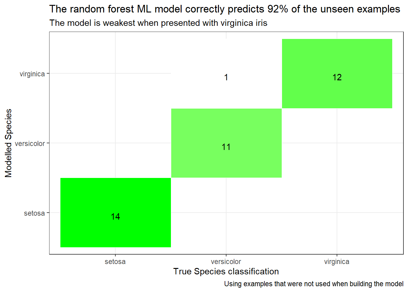
ML models can be quite difficult to understand. To adress this, the ML community have built a range of tools to help us inspect / understand what the model is doing and what inputs it things is most important to generate its outputs. The plot below shows the importance of the variables as far as this fitted random forest is concerned:
    #  the importance is here: model_clas_rf$variable.importance
model_clas_rf %>%
  vip::vip(num_features = 20,  aesthetics = list(color = "grey50", fill = "lightblue"))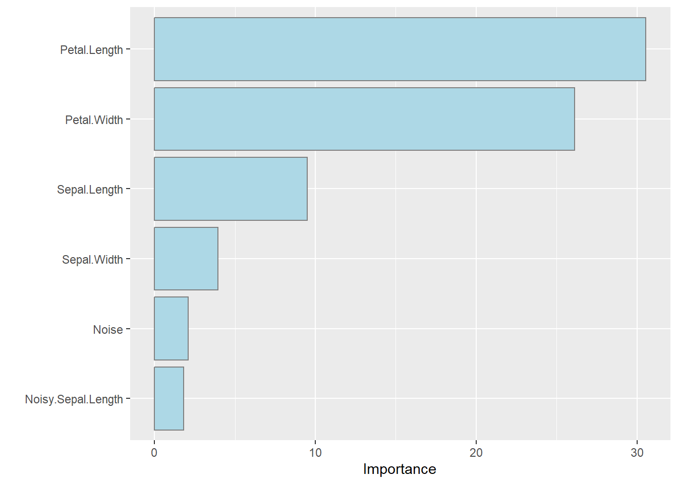
The variable importance plot shows that the Petal length and width are much more valuable to know when trying to classify the Species of an iris than (say) sepal dimensions, and even more valuable than those noisy measurements I added to the dataset which had little or no linkage with anything.
Actionable insight: The variable importance plots are valuable both:
to the model builder (to sense-check that the model is doing sensible things)
and for the process of data collection and retention… Why would you choose to purchase, collect and store the noise variable if it is not adding significant value to the decision making process?
Caveat: Take care when making value decisions. I would recommend testing model performance with and without the more exotic parameters in case they are rarely used, but super-valuable for some corner case that must be modelled well.
As described earlier, I’ve built the classification model on a random forest made up of 50 different decision trees. each decision tree is a family of nested IF-THEN statements that look a bit like that scooby-doo meme that started all of this.
We can inspect the contents of each tree as SQL (as shown below). SQL is really useful. We’re going to push the decision trees into Excel, but SQL can be pushed into databases so that the whole classification process can be done inside the database.
tidypredict::tidypredict_sql(model_clas_rf, dbplyr::simulate_dbi())[1] # SQL[[1]]
<SQL> CASE
WHEN (`Petal.Length` < 3.1 AND `Sepal.Width` >= 3.25) THEN 'setosa'
WHEN (`Petal.Length` < 2.45 AND `Petal.Length` < 4.95 AND `Sepal.Width` < 3.25) THEN 'setosa'
WHEN (`Sepal.Width` >= 2.75 AND `Petal.Length` >= 4.95 AND `Sepal.Width` < 3.25) THEN 'virginica'
WHEN (`Noise` < 0.308110165176913 AND `Petal.Length` >= 3.1 AND `Sepal.Width` >= 3.25) THEN 'versicolor'
WHEN (`Noise` >= 0.308110165176913 AND `Petal.Length` >= 3.1 AND `Sepal.Width` >= 3.25) THEN 'virginica'
WHEN (`Petal.Length` < 4.75 AND `Petal.Length` >= 2.45 AND `Petal.Length` < 4.95 AND `Sepal.Width` < 3.25) THEN 'versicolor'
WHEN (`Noisy.Sepal.Length` < 11.4622374536935 AND `Sepal.Width` < 2.75 AND `Petal.Length` >= 4.95 AND `Sepal.Width` < 3.25) THEN 'versicolor'
WHEN (`Noisy.Sepal.Length` >= 11.4622374536935 AND `Sepal.Width` < 2.75 AND `Petal.Length` >= 4.95 AND `Sepal.Width` < 3.25) THEN 'virginica'
WHEN (`Petal.Length` >= 4.85 AND `Sepal.Length` < 6.25 AND `Petal.Length` >= 4.75 AND `Petal.Length` >= 2.45 AND `Petal.Length` < 4.95 AND `Sepal.Width` < 3.25) THEN 'virginica'
WHEN (`Sepal.Width` >= 2.75 AND `Sepal.Length` >= 6.25 AND `Petal.Length` >= 4.75 AND `Petal.Length` >= 2.45 AND `Petal.Length` < 4.95 AND `Sepal.Width` < 3.25) THEN 'versicolor'
WHEN (`Sepal.Width` < 3.0 AND `Petal.Length` < 4.85 AND `Sepal.Length` < 6.25 AND `Petal.Length` >= 4.75 AND `Petal.Length` >= 2.45 AND `Petal.Length` < 4.95 AND `Sepal.Width` < 3.25) THEN 'virginica'
WHEN (`Sepal.Width` >= 3.0 AND `Petal.Length` < 4.85 AND `Sepal.Length` < 6.25 AND `Petal.Length` >= 4.75 AND `Petal.Length` >= 2.45 AND `Petal.Length` < 4.95 AND `Sepal.Width` < 3.25) THEN 'versicolor'
WHEN (`Noisy.Sepal.Length` < 15.3967564529274 AND `Sepal.Width` < 2.75 AND `Sepal.Length` >= 6.25 AND `Petal.Length` >= 4.75 AND `Petal.Length` >= 2.45 AND `Petal.Length` < 4.95 AND `Sepal.Width` < 3.25) THEN 'versicolor'
WHEN (`Noisy.Sepal.Length` >= 15.3967564529274 AND `Sepal.Width` < 2.75 AND `Sepal.Length` >= 6.25 AND `Petal.Length` >= 4.75 AND `Petal.Length` >= 2.45 AND `Petal.Length` < 4.95 AND `Sepal.Width` < 3.25) THEN 'virginica'
ENDThe above SQL works in databases but not in Excel. It’s not a huge leap of imagination to see how the WHEN statements could be converted into IF statements ready for Excel (more on this later).
Here’s what another tree in the forest looks like in SQL.
tidypredict::tidypredict_sql(model_clas_rf, dbplyr::simulate_dbi())[2] # SQL[[1]]
<SQL> CASE
WHEN (`Petal.Length` < 2.6 AND `Petal.Length` < 4.75) THEN 'setosa'
WHEN (`Petal.Width` >= 1.65 AND `Petal.Length` >= 4.75) THEN 'virginica'
WHEN (`Petal.Width` < 1.65 AND `Petal.Length` >= 2.6 AND `Petal.Length` < 4.75) THEN 'versicolor'
WHEN (`Petal.Width` >= 1.65 AND `Petal.Length` >= 2.6 AND `Petal.Length` < 4.75) THEN 'virginica'
WHEN (`Petal.Length` < 5.0 AND `Petal.Width` < 1.65 AND `Petal.Length` >= 4.75) THEN 'versicolor'
WHEN (`Petal.Length` >= 5.0 AND `Petal.Width` < 1.65 AND `Petal.Length` >= 4.75) THEN 'virginica'
ENDNotice that it is different (simpler in this case) and will give slightly different answers to the first. This is because it was trained on a different sub-set of the training data to the first. The second tree also uses “Noisy.Sepal.Length” (and an apparently extremely precise number as a threshold). We knew at the outset that “Noisy.Sepal.Length” is a red-herring (I deliberately created it as a corrupted version of Sepal.Length). Perhaps it’s a surprise that it was included, but there’s manifestly some value in it when the options are sufficiently limited. In general we don’t know at the outset which variables hold insight into out problem, however, the variable importance plot has shown us that overall it is not as valuable as some other variables. If we had access to a domain expert, perhaps we would ask them whether there is any real value in this measurement. Perhaps we would explore a new cut of the iris dataset that excluded “Noisy.Sepal.Length” (and Noise) based on the variable importance plot . After this review of the results we might choose to not use these variables. I’m not going to do any if this as it’s not material to this expo.
I’ve written a couple of functions that will take the logic formatted as SQL and turn it into something that can be run in Excel (see folded code below):
#' @title sql_to_excel
#'
#' @description
#' This function converts a string as outputted by tidymodels::tidypredict_sql()
#' and returns something that model like an Excel formula
#' the result includes variable (column) names,  not cell references
#' @param trees_df a 1D df containing one row per model
#' @param input_df The dataframe upon which the model is to be used
#' @param n_sf number of significant figures (parameters are rounded to save space)
#' @param squishit should extra whitespace be removed to save space
#'
#' @return a dataframe with the reformatted equation(s) in rows
#'
#' @export
#'
sql_to_excel <- function(trees_df, input_df, n_sf = 3, squishit = T) {

  # sorry in advance for using a for loop!
  # xgboost model always includes a null check
  # e.g. CASE\nWHEN ((`Petal.Width` < 0.800000012 OR (`Petal.Width` IS NULL))) THEN 0.282941192
  # I want to remove all insances of  OR (`Petal.Width` IS NULL) (for all potential variables)
  for (col_name in names(input_df)) {
    trees_df <- trees_df %>%
#      " OR \\(`Petal.Width` IS NULL\\)"
      mutate(instruction = str_remove_all(instruction, paste0(" OR \\(`", col_name, "` IS NULL\\)")))
  }

  if(F) {
    # one last bit
    trees_df <- trees_df %>%
      # we dont need any 0.0 + lines
      mutate(instruction = str_remove_all(instruction, "0.0 \\+ "))

  }

  equations_in_cols_a <- trees_df %>%
    # adapt
    # the kinds of things you find output from tidypredict_sql
    mutate(instruction = paste0("=", instruction)) %>%
    mutate(instruction = str_replace_all(instruction, "AND", ",")) %>%
    mutate(instruction = str_replace_all(instruction, "CASE\nWHEN", "IF(AND")) %>%
    mutate(n_parts = str_count(instruction, "\n"), .before = instruction) %>%
    mutate(instruction = str_replace_all(instruction, "WHEN", ", IF(AND")) %>%
    mutate(instruction = str_replace_all(instruction, "THEN", ", ")) %>%
    mutate(instruction = str_replace_all(instruction, "END", ", 'SHOULDNTHAPPEN'")) %>%
    mutate(end = str_pad(string = "", width = n_parts, side = "right", pad = ")"), .after = n_parts) %>%
    mutate(output = paste0(instruction, end)) %>%
    mutate(output = str_replace_all(output, "'", '"')) %>%
    mutate(output = str_squish(output))

  # limit to a certain number of significant figures
  if(exists("n_sf")) {
    equations_in_cols_a <- equations_in_cols_a  %>%
      mutate(output = str_replace_all(output, "\\d+\\.\\d+", function(x) as.character(round(as.numeric(x), n_sf))))
  }

  # remove any unnecessary spaces that are only really there to aid the human eye
  if(squishit) {
    equations_in_cols_a <- equations_in_cols_a  %>%
      mutate(output = str_replace_all(output, " ", ""))
  }

  # we are going to swap references to the column names in R
  # with column names in Excel (e.g. Sepal.Width becomes A[ROW_NUM])
  # we're adding [ROW_NUM] because later we're going to have many rows of calcs
  # substitute A[ROW_NUM], with A[1], A[2] etc.
  # this dataframe has two columns,  the R column name and the A/B/C etc for Excel
  # we'll subsitute the R ones with th Excel cols references later
  replacements <- names(input_df) %>%
    tolower() %>%
    enframe(name = NULL, value = "word") %>%
    mutate(col_letter = paste0(LETTERS[row_number()], "[ROW_NUM]"))

  # ultimately we'll be having one equation per column
  # for now there's one equation per row
  # we're going to want to labels them rule_1...rule_n
  # (these will be the col titles) in Excel)
  # AND ...
  # we want to substitute the original variable names in the equations
  # with the corresponding Excel column references
  equations_in_cols <- equations_in_cols_a %>%
    # make a reference to the column names...
    mutate(tree_number = row_number()) %>%
    # unpack the (wide) equation into (long) parts so we can get at the variables
    tidytext::unnest_tokens(word, output, token = "regex", pattern = "`") %>%
    # we only need a couple of the columns going forwards
    select(tree_number, word) %>%
    # do a lookup find&replace using left_join
    left_join(replacements)

  # breakpoint in the pipeline here.. .I want to check that some of the
  # variables have been found
  # (i.e. we're not passing in a dataframe that doesnt have the same variables)
  if(nrow(equations_in_cols %>% filter(!is.na(col_letter))) <1) {
    warning("sql_to_excel: NO MATCHES IN replacements")
  } else {
    message("sql_to_excel: replacements found")
  }

  equations_in_cols <- equations_in_cols %>%
    # then coalesce, as this will sub-in col_letter is it's defined, and word if not
    mutate(new_word = coalesce(col_letter, word)) %>%
    # now we can repack the (long) parts of the equations into whole (wide) equation
    # grouping by tree_number will work on all the components of each equation in turn
    group_by(tree_number) %>%
    # summarise paste0 concatenates the rows into one (wide) reconstructed equation
    summarise(output = paste0(new_word, collapse = ''))

  #| transpose (flip) the array so that
  #| the equations are in columns rather than rows
  equations_in_rows <- equations_in_cols %>%
#    mutate(tree_number = paste0("tree_", tree_number)) %>%
    gather(key = var_name, value = value, 2:ncol(equations_in_cols)) %>%
    spread(key = names(equations_in_cols)[1],value = 'value') %>%
    rename_with(~ paste0("tree_", .), -var_name) %>%
    select(-var_name)

  return(equations_in_rows)
}
The function generates the following output for the tree we have been exploring. Those familiar with Excel cell formulae will see that this is getting close to something usable inside Excel.
#| random forest classification in Excel format ----
# tidypredict_sql takes a while (10s of seconds)
trees_df_iris_rf_clas <- tidypredict::tidypredict_sql(model_clas_rf, dbplyr::simulate_dbi()) %>%
  tibble::enframe(name = NULL, value = "instruction") %>%
  mutate(instruction = unlist(instruction))

randforest_clas <- sql_to_excel(trees_df = trees_df_iris_rf_clas, input_df = iris_n_noise)

randforest_clas$tree_1
[1] "=if(and(C[ROW_NUM]<3.1,B[ROW_NUM]>=3.25),\"setosa\",if(and(C[ROW_NUM]<2.45,C[ROW_NUM]<4.95,B[ROW_NUM]<3.25),\"setosa\",if(and(B[ROW_NUM]>=2.75,C[ROW_NUM]>=4.95,B[ROW_NUM]<3.25),\"virginica\",if(and(F[ROW_NUM]<0.308,C[ROW_NUM]>=3.1,B[ROW_NUM]>=3.25),\"versicolor\",if(and(F[ROW_NUM]>=0.308,C[ROW_NUM]>=3.1,B[ROW_NUM]>=3.25),\"virginica\",if(and(C[ROW_NUM]<4.75,C[ROW_NUM]>=2.45,C[ROW_NUM]<4.95,B[ROW_NUM]<3.25),\"versicolor\",if(and(G[ROW_NUM]<11.462,B[ROW_NUM]<2.75,C[ROW_NUM]>=4.95,B[ROW_NUM]<3.25),\"versicolor\",if(and(G[ROW_NUM]>=11.462,B[ROW_NUM]<2.75,C[ROW_NUM]>=4.95,B[ROW_NUM]<3.25),\"virginica\",if(and(C[ROW_NUM]>=4.85,A[ROW_NUM]<6.25,C[ROW_NUM]>=4.75,C[ROW_NUM]>=2.45,C[ROW_NUM]<4.95,B[ROW_NUM]<3.25),\"virginica\",if(and(B[ROW_NUM]>=2.75,A[ROW_NUM]>=6.25,C[ROW_NUM]>=4.75,C[ROW_NUM]>=2.45,C[ROW_NUM]<4.95,B[ROW_NUM]<3.25),\"versicolor\",if(and(B[ROW_NUM]<3,C[ROW_NUM]<4.85,A[ROW_NUM]<6.25,C[ROW_NUM]>=4.75,C[ROW_NUM]>=2.45,C[ROW_NUM]<4.95,B[ROW_NUM]<3.25),\"virginica\",if(and(B[ROW_NUM]>=3,C[ROW_NUM]<4.85,A[ROW_NUM]<6.25,C[ROW_NUM]>=4.75,C[ROW_NUM]>=2.45,C[ROW_NUM]<4.95,B[ROW_NUM]<3.25),\"versicolor\",if(and(G[ROW_NUM]<15.397,B[ROW_NUM]<2.75,A[ROW_NUM]>=6.25,C[ROW_NUM]>=4.75,C[ROW_NUM]>=2.45,C[ROW_NUM]<4.95,B[ROW_NUM]<3.25),\"versicolor\",if(and(G[ROW_NUM]>=15.397,B[ROW_NUM]<2.75,A[ROW_NUM]>=6.25,C[ROW_NUM]>=4.75,C[ROW_NUM]>=2.45,C[ROW_NUM]<4.95,B[ROW_NUM]<3.25),\"virginica\",\"shouldnthappen\"))))))))))))))"Note some of the things the function has done:
Convert SQL / DPLYR conditional logic to Excel-friendly IF() logic. This is necessary to allow Excel to evaluate the decision tree natively.
Convert dataset column names into row-col cell references. The dataset columns start as “A” and progress up the alphabet. The columns count up from the first row of data (starting at row 2 as the data I eventually push into Excel will have the variable names in the first column). At this point in the process I’m just putting “ROW_NUM” as a place-holder for the real row-number as the formula is yet to be added as a column next to the iris dataset. I’ll replace ROW_NUM with 2, 3 etc when I add the formula to each row of the dataset in Excel.
Limit the number of significant figures for the condition thresholds. This is a practical step to limit the length of the logic representing the decision trees in each Excel cell and may be configures to higher resolution if required.
For example:
WHEN (`Noise` < 0.0444393495563418 AND `Sepal.Width` < 3.35) THEN 'virginica'
becomes
=if(and(F[ROW_NUM]<0.044,B[ROW_NUM]<3.35),\"virginica\"
We’re almost there! The process of fitting Machine Learning models and preparing them to be used inside Excel is starting to come together. The above is the logic from just one of the 50 decision trees. Each of the other trees was trained on slightly different data and hence has captured slightly different logic. All trees are of value and must be translated and exported. When resolving different suggestions for Species from different trees, the random forest algorithms can use voting methods like “most often suggested” to come up with a single final answer. If I’m to get this embedding into Excel I will have to emulate the voting system too. See the section on getting the models into Excel for the rest of that story. For now I’ll move on to regression.
I’m re-using the iris dataset to explore regression. In this section, instead of having the Species as a target variable, I’m going to model Petal.Length. I’ll be making available all the other stuff I know about each iris to the learning systems. They will pick and choose which variables are important and how they should be combined to give me a way of estimating how long my iris petals might be given all that other information.
Random forests are a form of ML that can do both classification AND regression. This is great because most of what I’ve written, and you’ve read from the classification section remains true9.
Before diving in to random forests for regression I thought I’d have a quick look at a more traditional way of building regression models…. Linear regression.
First off, I’d just like to state that linear models and generalised linear models are a form of machine learning. They generate information from data. I’m deliberately(ish) adding this section on regression in LMs because they are more familiar to many than other ML techniques and act as a valuable reference to compare other ML techniques against. And yes, I appreciate that Excel already has capability to do linear regression, but I’m trying to highlight bridges here.
Fitting linear models in R and checking the significance of each parameter is really easy.
model_reg_lm <- lm(Petal.Length ~ ., data=df_train)
model_reg_lm
Call:
lm(formula = Petal.Length ~ ., data = df_train)

Coefficients:
       (Intercept)        Sepal.Length         Sepal.Width         Petal.Width
         -1.273048            0.642512           -0.167031            0.596730
 Speciesversicolor    Speciesvirginica               Noise  Noisy.Sepal.Length
          1.428322            1.941926           -0.121968            0.001561
We can follow standard processes and inspect the significance of each parameter:
model_reg_lm %>%
    broom::tidy() %>% arrange(p.value)
# A tibble: 8 × 5
term estimate std.error statistic p.value
<chr> <dbl> <dbl> <dbl> <dbl>
1 Sepal.Length 0.643 0.0594 10.8 9.65e-19
2 Speciesversicolor 1.43 0.201 7.12 1.46e-10
3 Speciesvirginica 1.94 0.281 6.91 3.97e-10
4 Petal.Width 0.597 0.147 4.06 9.46e- 5
5 (Intercept) -1.27 0.325 -3.92 1.59e- 4
6 Sepal.Width -0.167 0.0961 -1.74 8.51e- 2
7 Noise -0.122 0.0861 -1.42 1.59e- 1
8 Noisy.Sepal.Length 0.00156 0.00966 0.161 8.72e- 1Reassuringly, the Noise & “Noisy.Sepal.Length” measurements are flagged as the least significant measurements in the model.
We can refine the model to only include useful stuff by step-wise variable selection…
model_reg_lm_simplified <- MASS::stepAIC(model_reg_lm, direction = "both", trace = FALSE)
# have a look at this model
model_reg_lm_simplified %>%
  broom::tidy() %>% arrange(p.value)
# A tibble: 7 × 5
term estimate std.error statistic p.value
<chr> <dbl> <dbl> <dbl> <dbl>
1 Sepal.Length 0.645 0.0578 11.2 1.58e-19
2 Speciesversicolor 1.43 0.199 7.18 1.04e-10
3 Speciesvirginica 1.95 0.279 6.99 2.68e-10
4 Petal.Width 0.594 0.145 4.09 8.36e- 5
5 (Intercept) -1.26 0.315 -4.00 1.17e- 4
6 Sepal.Width -0.169 0.0951 -1.77 7.89e- 2
7 Noise -0.122 0.0856 -1.42 1.59e- 1Step-wise regression generates a simpler model (which could be further refined). Notice that some parameters that were retained in the simplification process are not significant at p<0.05).
The model that has been allowed to add & remove variables is simpler and better than the model forced to use all of the variables. The comparison below shows that the same accuracy can be achieved with fewer parameters:
performance::compare_performance(model_reg_lm, model_reg_lm_simplified, rank = TRUE)# Comparison of Model Performance Indices
Name | Model | R2 | R2 (adj.) | RMSE | Sigma | AIC weights | AICc weights | BIC weights | Performance-Score
----------------------------------------------------------------------------------------------------------------------------------
model_reg_lm_simplified | lm | 0.978 | 0.977 | 0.261 | 0.270 | 0.728 | 0.763 | 0.913 | 71.43%
model_reg_lm | lm | 0.978 | 0.977 | 0.261 | 0.271 | 0.272 | 0.237 | 0.087 | 28.57%Let’s check how well the models perform on the test data:
# creating ggplot object for visualization
df_test %>%
  bind_cols(predict(model_reg_lm, df_test) %>%
              enframe(name = NULL, value = "full_prediction")
            ) %>%
  bind_cols(predict(model_reg_lm_simplified, df_test) %>%
              enframe(name = NULL, value = "simplified_prediction")
            ) %>%
  select(Petal.Length, Species, full_prediction, simplified_prediction) %>%
  pivot_longer(-c(Petal.Length, Species), names_to = "model", values_to = "estimate") %>%
  ggplot(aes(Petal.Length, estimate)) +
  geom_point(aes(colour = Species)) +
  ggpubr::stat_regline_equation(aes(label =  paste(after_stat(eq.label),
                                                   after_stat(adj.rr.label), sep = "~~~~"))) +
  geom_smooth(method = "lm") +
  facet_wrap( ~ model) +
  labs(title = "Both the full linear model and the simpler one look good",
       subtitle = "This plot is based on the test dataset",
       x = "True Petal Length",
       y = "Modelled Petal Length")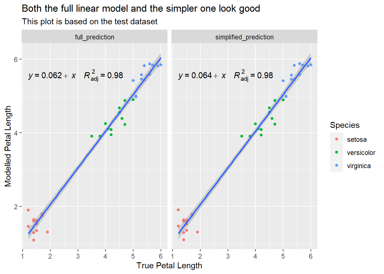
The model can be turned into something that can be used in R code:
tidypredict::tidypredict_fit(model_reg_lm_simplified)-1.26135667586224 + (Sepal.Length * 0.64450799017439) + (Sepal.Width *
-0.168701458745407) + (Petal.Width * 0.593689001666243) +
(ifelse(Species == "versicolor", 1, 0) * 1.43053323954197) +
(ifelse(Species == "virginica", 1, 0) * 1.94595745930648) +
(Noise * -0.1215414770554)… and translated into something that looks more like something Excel would recognise:
#' @title fit_to_excel
#'
#' @description
#' This function converts a string as outputted by tidymodels::tidypredict_fit()
#' and returns something that model like an Excel formula
#' the result includes variable (column) names,  not cell references
#' @param trees_df a 1D df containing one row per model
#' @param input_df The dataframe upon which the model is to be used
#' @param n_sf number of significant figures (parameters are rounded to save space)
#' @param squishit should extra whitespace be removed to save space
#'
#' @return a dataframe with the reformatted equation(s) in rows
#'
#' @export
#'
fit_to_excel <- function(trees_df, input_df, n_sf = 3, squishit = T) {

  equations_in_cols_a <- trees_df %>%
    # adapt
    # the kinds of things you find output from tidypredict_fit
    mutate(output = instruction) %>%
    mutate(output = str_replace_all(output, "ifelse", "if")) %>%
    mutate(output = str_replace_all(output, "==", "=")) %>%
    mutate(output = str_squish(output))

  # limit to a certain number of significant figures
  if(exists("n_sf")) {
    equations_in_cols_a <- equations_in_cols_a  %>%
      mutate(output = str_replace_all(output, "\\d+\\.\\d+", function(x) as.character(round(as.numeric(x), n_sf))))
  }

  # remove any unnecessary spaces that are only really there to aid the human eye
  if(squishit) {
    equations_in_cols_a <- equations_in_cols_a  %>%
      mutate(output = str_replace_all(output, " ", "")) %>%
      mutate(output_as_excel = "") # im adding this so I can check works been done
  }

  # we are going to swap references to the column names in R
  # with column names in Excel (e.g. Sepal.Width becomes A[ROW_NUM])
  # we're adding [ROW_NUM] because later we're going to have many rows of calcs
  # substitute A[ROW_NUM], with A[1], A[2] etc.
  # this dataframe has two columns,  the R column name and the A/B/C etc for Excel
  # we'll subsitute the R ones with th Excel cols references later
  replacements <- names(input_df) %>%
    enframe(name = NULL, value = "word") %>%
    mutate(col_letter = paste0(LETTERS[row_number()], "[ROW_NUM]"))

  # ultimately we'll be having one equation per column
  # for now there's one equation per row
  # we're going to want to labels them rule_1...rule_n
  # (these will be the col titles) in Excel)
  # AND ...
  # we want to substitute the original variable names in the equations
  # with the corresponding Excel column references
  # stack exchange to the rescue:
  # https://stackoverflow.com/questions/50750266/r-find-and-replace-partial-string-based-on-lookup-table
  for(i in 1:nrow(equations_in_cols_a)) {
    orig_row <- equations_in_cols_a[i,]$output
#    print(as.character(row))
    updated_row <- stringi::stri_replace_all_fixed(orig_row, replacements$word, replacements$col_letter, vectorize_all=FALSE)
#    print(row)
    equations_in_cols_a[i,]$output_as_excel <- updated_row
  }
  if( nrow(equations_in_cols_a %>% filter(output == output_as_excel)) ) {
    warning("fit_to_excel: NO MATCHES IN replacements")
  } else {
    message("fit_to_excel: replacements found")
  }

  equations_in_cols <- equations_in_cols_a %>%
    transmute(output = output_as_excel) %>%
    mutate(tree_number = row_number(), .before = 1)
  #| transpose (flip) the array so that
  #| the equations are in columns rather than rows
  equations_in_rows <- equations_in_cols %>%
    select(output) %>%
    mutate(tree_number = row_number(), .before = 1) %>%
    gather(key = var_name, value = value, 2:ncol(equations_in_cols)) %>%
    spread(key = names(equations_in_cols)[1],value = 'value') %>%
    rename_with(~ paste0("tree_", .), -var_name) %>%
    select(-var_name)

  return(equations_in_rows)
} #
  # this emulates LM in Excel format ----
  trees_df_lm <- tidypredict::tidypredict_fit(model_reg_lm)[2] %>% as.character() %>%
    tibble::enframe(name = NULL, value = "instruction") %>%
    mutate(instruction = unlist(instruction)) %>%
    mutate(instruction = as.character(instruction))

lm_excel <- fit_to_excel(trees_df = trees_df_lm, input_df = iris_n_noise)
fit_to_excel: replacements foundas.character(lm_excel)[1] "-1.273+(A[ROW_NUM]*0.643)+(B[ROW_NUM]*-0.167)+(D[ROW_NUM]*0.597)+(if(E[ROW_NUM]=\"versicolor\",1,0)*1.428)+(if(E[ROW_NUM]=\"virginica\",1,0)*1.942)+(F[ROW_NUM]*-0.122)"As stated previously, random forests can be used for both classification and regression tasks with very little modification. Regression random forests can have bigger trees with more leaves, and the suggestions from all the individual trees are reconciled by using averages rather than the majority voting method described for classification, but most of the mechanics remain unaltered when using them for regression.
I’m going to make one minor modification to the Iris dataset before feeding it into the random forest for regression. I’m going to change the way that Species is encoded. I’ll change it from three words, to three numbers. Note: if you’re going to use this code to firt your own dataset then you will have to convert any factors or strings into integers as I have, and adapt the regression equation to ignore the originals. This is the only compromise I’m making in this post and I’m going to do so because I’m relying on a routine called tidypredict::tidypredict_sql() to flatten the decision tree rules and convert them into SQL. this routine returns the logic for factors (like Species) as numbers, so it’s easier for me to turn them into numbers at the outset than handle the mapping when I return the SQL. The code to re-map the Species is shown below:
iris_n_noise_reg <- iris_n_noise %>%
  mutate(Species_n = as.integer(Species), .after = Species)
# As before, the avoid over-fitting,  I'll split the regression dataset into training and testing datasets. First I'll split the data into two (one set is something I can use to train the model,  the other I will keep in reserve to test the model.  Then, I will build a 10-fold cross-validation dataset from training dataset. This sounds fancy, but it's just creating 10 alternative takes on the iris dataset by sampling (with replacement) from the initial one. All 10 folds contain examples drawn from the iris dataset, but each fold will contain a different mix of examples

set.seed(037)
iris_reg_split <- rsample::initial_split(iris_n_noise_reg, strata = Petal.Length)
iris_reg_train <- rsample::training(iris_reg_split)
iris_reg_test <-  rsample::testing(iris_reg_split)
Now I can build the random forest:
set.seed(37) # setting a seed helps with reproducibility
# we're modelling Species as a function of everything...
model_reg_rf <- ranger::ranger(Petal.Length ~ . - Species,
                    data = iris_reg_train,
                    num.trees = ntrees_reg_rf,
                    # I've added the optional impurity
                    # so I check variable importance later
                    importance = "impurity"
)
model_reg_rf
Ranger result
Call:
ranger::ranger(Petal.Length ~ . - Species, data = iris_reg_train, num.trees = ntrees_reg_rf, importance = "impurity")
Type: Regression
Number of trees: 50
Sample size: 111
Number of independent variables: 6
Mtry: 2
Target node size: 5
Variable importance mode: impurity
Splitrule: variance
OOB prediction error (MSE): 0.1077428
R squared (OOB): 0.964898 It’s always a good idea to plot the model’s performance:
# then do a quick check on the output
pred.iris_rf <- stats::predict(model_reg_rf, data = iris_reg_test)
bind_cols(iris_reg_test$Petal.Length, pred.iris_rf$predictions) %>%
  rename(actual = ...1, pred = ...2) %>%
  ggplot(aes(actual, pred)) +
  geom_point() +
  ggpubr::stat_regline_equation(aes(label =  paste(after_stat(eq.label),
                                                   after_stat(adj.rr.label), sep = "~~~~")), size = 4) +
  geom_smooth(method = "lm") +
  geom_abline(slope = 1, intercept = 0) +
  labs(title = "The random forest model is good a predicting Petal.Length",
     subtitle = "This plot shows performance on unseen data",
     x = "Actual Petal Length", y = "Model estimate of Petal Length")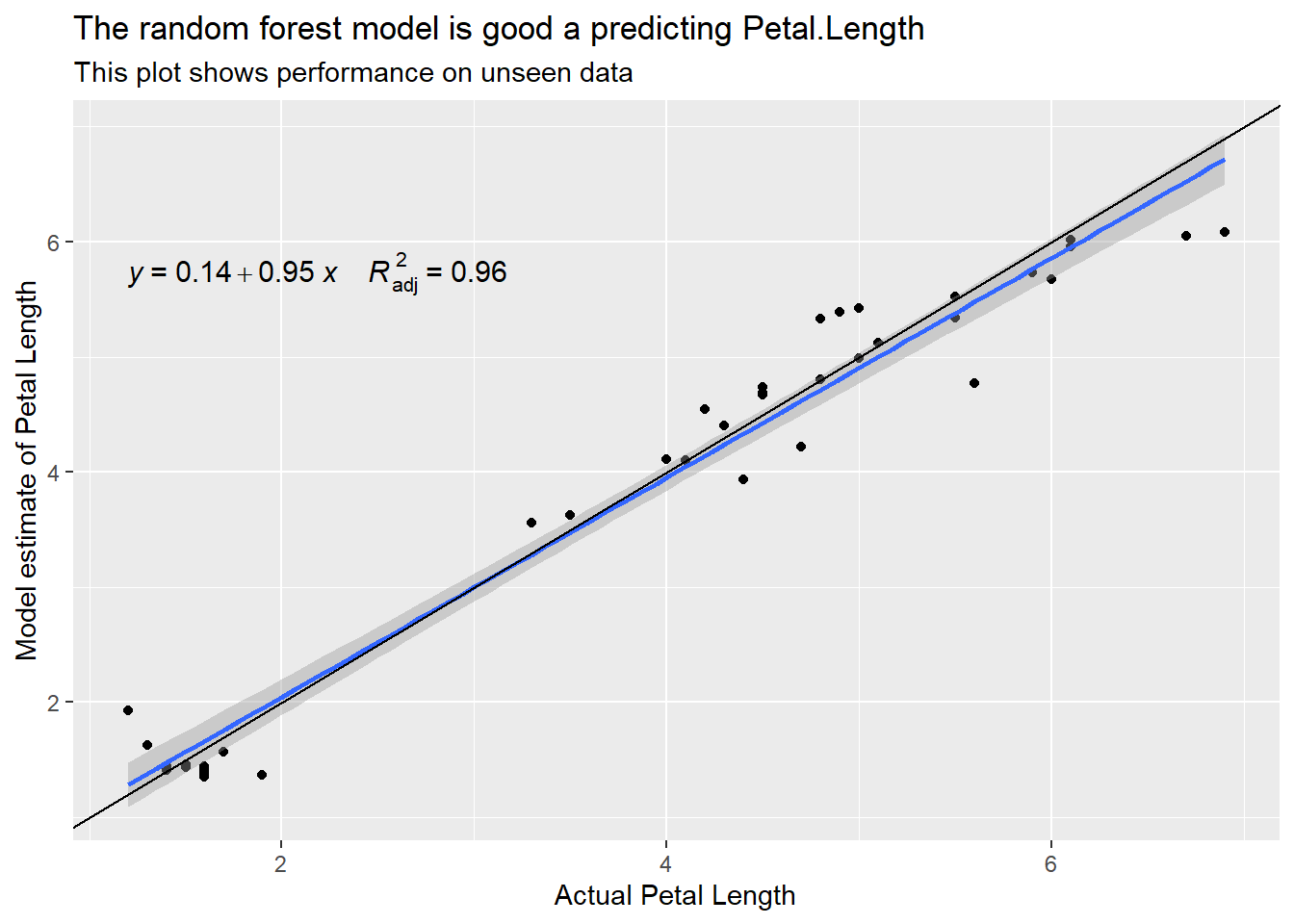
… and check what variables are considered important in this model:
model_reg_rf %>%
      vip::vip(num_features = 20,  aesthetics = list(color = "grey50", fill = "lightblue"))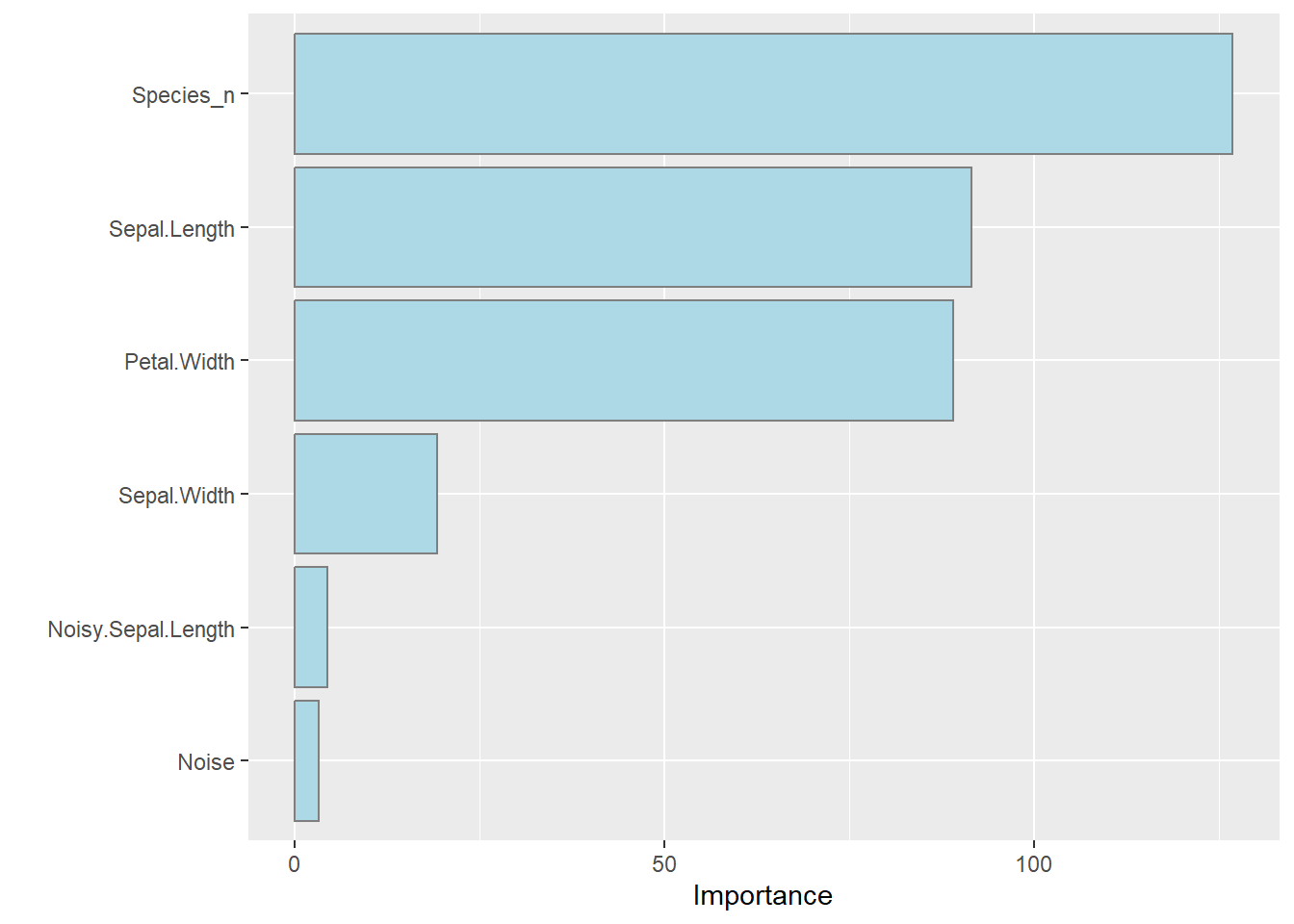
Species_n is the integer version of the Species. When building the model I asked it to use Species_n rather than Species. The random forest finds that Species_n, Sepal.Length and Petal.With are most useful when estimating the length of the petals.
Then carry on having extracted the rules as per the classification example. See below for a single tree from the random forest. Notice that the tree is considerably larger than the one we explored in the classification case.
tidypredict::tidypredict_sql(model_reg_rf, dbplyr::simulate_dbi())[1][[1]]
<SQL> CASE
WHEN (`Noisy.Sepal.Length` >= 14.6750497869682 AND `Sepal.Width` >= 3.35) THEN 5.6
WHEN (`Petal.Width` >= 0.75 AND `Sepal.Length` < 5.15 AND `Sepal.Width` < 3.35) THEN 4.1
WHEN (`Petal.Width` >= 1.3 AND `Noisy.Sepal.Length` < 14.6750497869682 AND `Sepal.Width` >= 3.35) THEN 6.25
WHEN (`Noisy.Sepal.Length` < 5.3814420059789 AND `Petal.Width` < 0.75 AND `Sepal.Length` < 5.15 AND `Sepal.Width` < 3.35) THEN 1.7
WHEN (`Sepal.Length` < 4.95 AND `Petal.Width` < 1.3 AND `Noisy.Sepal.Length` < 14.6750497869682 AND `Sepal.Width` >= 3.35) THEN 1.4
WHEN (`Petal.Width` >= 1.35 AND `Noisy.Sepal.Length` < 12.8900942521635 AND `Petal.Width` < 1.45 AND `Sepal.Length` >= 5.15 AND `Sepal.Width` < 3.35) THEN 4.45
WHEN (`Noise` < 0.33885505865328 AND `Noisy.Sepal.Length` >= 12.8900942521635 AND `Petal.Width` < 1.45 AND `Sepal.Length` >= 5.15 AND `Sepal.Width` < 3.35) THEN 3.9
WHEN (`Noise` < 0.0792251240927726 AND `Petal.Width` < 2.05 AND `Petal.Width` >= 1.45 AND `Sepal.Length` >= 5.15 AND `Sepal.Width` < 3.35) THEN 4.5
WHEN (`Noisy.Sepal.Length` >= 13.9618772745132 AND `Sepal.Length` >= 4.95 AND `Petal.Width` < 1.3 AND `Noisy.Sepal.Length` < 14.6750497869682 AND `Sepal.Width` >= 3.35) THEN 1.9
WHEN (`Sepal.Width` < 3.1 AND `Noise` < 0.29474036488682 AND `Noisy.Sepal.Length` >= 5.3814420059789 AND `Petal.Width` < 0.75 AND `Sepal.Length` < 5.15 AND `Sepal.Width` < 3.35) THEN 1.23333333333333
WHEN (`Sepal.Width` >= 3.1 AND `Noise` < 0.29474036488682 AND `Noisy.Sepal.Length` >= 5.3814420059789 AND `Petal.Width` < 0.75 AND `Sepal.Length` < 5.15 AND `Sepal.Width` < 3.35) THEN 1.33333333333333
WHEN (`Noisy.Sepal.Length` < 11.1026142048649 AND `Noise` >= 0.29474036488682 AND `Noisy.Sepal.Length` >= 5.3814420059789 AND `Petal.Width` < 0.75 AND `Sepal.Length` < 5.15 AND `Sepal.Width` < 3.35) THEN 1.5
WHEN (`Noisy.Sepal.Length` >= 11.1026142048649 AND `Noise` >= 0.29474036488682 AND `Noisy.Sepal.Length` >= 5.3814420059789 AND `Petal.Width` < 0.75 AND `Sepal.Length` < 5.15 AND `Sepal.Width` < 3.35) THEN 1.43333333333333
WHEN (`Sepal.Length` >= 5.65 AND `Petal.Width` < 1.35 AND `Noisy.Sepal.Length` < 12.8900942521635 AND `Petal.Width` < 1.45 AND `Sepal.Length` >= 5.15 AND `Sepal.Width` < 3.35) THEN 4.08
WHEN (`Sepal.Width` >= 3.0 AND `Noise` >= 0.33885505865328 AND `Noisy.Sepal.Length` >= 12.8900942521635 AND `Petal.Width` < 1.45 AND `Sepal.Length` >= 5.15 AND `Sepal.Width` < 3.35) THEN 4.4
WHEN (`Species_n` < 2.5 AND `Noise` >= 0.0792251240927726 AND `Petal.Width` < 2.05 AND `Petal.Width` >= 1.45 AND `Sepal.Length` >= 5.15 AND `Sepal.Width` < 3.35) THEN 4.95
WHEN (`Noisy.Sepal.Length` < 6.96604795712046 AND `Sepal.Width` < 3.15 AND `Petal.Width` >= 2.05 AND `Petal.Width` >= 1.45 AND `Sepal.Length` >= 5.15 AND `Sepal.Width` < 3.35) THEN 5.8
WHEN (`Noisy.Sepal.Length` < 11.7626817545388 AND `Sepal.Width` >= 3.15 AND `Petal.Width` >= 2.05 AND `Petal.Width` >= 1.45 AND `Sepal.Length` >= 5.15 AND `Sepal.Width` < 3.35) THEN 5.7
WHEN (`Noisy.Sepal.Length` >= 11.7626817545388 AND `Sepal.Width` >= 3.15 AND `Petal.Width` >= 2.05 AND `Petal.Width` >= 1.45 AND `Sepal.Length` >= 5.15 AND `Sepal.Width` < 3.35) THEN 5.95
WHEN (`Noisy.Sepal.Length` >= 11.3397545781452 AND `Sepal.Length` < 5.65 AND `Petal.Width` < 1.35 AND `Noisy.Sepal.Length` < 12.8900942521635 AND `Petal.Width` < 1.45 AND `Sepal.Length` >= 5.15 AND `Sepal.Width` < 3.35) THEN 4.1
WHEN (`Noise` < 0.622111424105242 AND `Sepal.Width` < 3.0 AND `Noise` >= 0.33885505865328 AND `Noisy.Sepal.Length` >= 12.8900942521635 AND `Petal.Width` < 1.45 AND `Sepal.Length` >= 5.15 AND `Sepal.Width` < 3.35) THEN 4.7
WHEN (`Noise` >= 0.622111424105242 AND `Sepal.Width` < 3.0 AND `Noise` >= 0.33885505865328 AND `Noisy.Sepal.Length` >= 12.8900942521635 AND `Petal.Width` < 1.45 AND `Sepal.Length` >= 5.15 AND `Sepal.Width` < 3.35) THEN 4.6
WHEN (`Noise` < 0.477415315923281 AND `Species_n` >= 2.5 AND `Noise` >= 0.0792251240927726 AND `Petal.Width` < 2.05 AND `Petal.Width` >= 1.45 AND `Sepal.Length` >= 5.15 AND `Sepal.Width` < 3.35) THEN 5.3
WHEN (`Noise` >= 0.903480604640208 AND `Noisy.Sepal.Length` >= 6.96604795712046 AND `Sepal.Width` < 3.15 AND `Petal.Width` >= 2.05 AND `Petal.Width` >= 1.45 AND `Sepal.Length` >= 5.15 AND `Sepal.Width` < 3.35) THEN 5.1
WHEN (`Noisy.Sepal.Length` < 8.82421281863935 AND `Sepal.Width` < 3.45 AND `Noisy.Sepal.Length` < 13.9618772745132 AND `Sepal.Length` >= 4.95 AND `Petal.Width` < 1.3 AND `Noisy.Sepal.Length` < 14.6750497869682 AND `Sepal.Width` >= 3.35) THEN 1.5
WHEN (`Noisy.Sepal.Length` >= 8.82421281863935 AND `Sepal.Width` < 3.45 AND `Noisy.Sepal.Length` < 13.9618772745132 AND `Sepal.Length` >= 4.95 AND `Petal.Width` < 1.3 AND `Noisy.Sepal.Length` < 14.6750497869682 AND `Sepal.Width` >= 3.35) THEN 1.65
WHEN (`Noise` < 0.100762510555796 AND `Sepal.Width` >= 3.45 AND `Noisy.Sepal.Length` < 13.9618772745132 AND `Sepal.Length` >= 4.95 AND `Petal.Width` < 1.3 AND `Noisy.Sepal.Length` < 14.6750497869682 AND `Sepal.Width` >= 3.35) THEN 1.575
WHEN (`Noisy.Sepal.Length` < 7.5022319547832 AND `Noisy.Sepal.Length` < 11.3397545781452 AND `Sepal.Length` < 5.65 AND `Petal.Width` < 1.35 AND `Noisy.Sepal.Length` < 12.8900942521635 AND `Petal.Width` < 1.45 AND `Sepal.Length` >= 5.15 AND `Sepal.Width` < 3.35) THEN 4.0
WHEN (`Sepal.Length` >= 6.2 AND `Noise` >= 0.477415315923281 AND `Species_n` >= 2.5 AND `Noise` >= 0.0792251240927726 AND `Petal.Width` < 2.05 AND `Petal.Width` >= 1.45 AND `Sepal.Length` >= 5.15 AND `Sepal.Width` < 3.35) THEN 5.12
WHEN (`Sepal.Length` < 6.1 AND `Noise` < 0.903480604640208 AND `Noisy.Sepal.Length` >= 6.96604795712046 AND `Sepal.Width` < 3.15 AND `Petal.Width` >= 2.05 AND `Petal.Width` >= 1.45 AND `Sepal.Length` >= 5.15 AND `Sepal.Width` < 3.35) THEN 5.1
WHEN (`Sepal.Length` >= 6.1 AND `Noise` < 0.903480604640208 AND `Noisy.Sepal.Length` >= 6.96604795712046 AND `Sepal.Width` < 3.15 AND `Petal.Width` >= 2.05 AND `Petal.Width` >= 1.45 AND `Sepal.Length` >= 5.15 AND `Sepal.Width` < 3.35) THEN 5.56
WHEN (`Sepal.Length` < 5.05 AND `Noise` >= 0.100762510555796 AND `Sepal.Width` >= 3.45 AND `Noisy.Sepal.Length` < 13.9618772745132 AND `Sepal.Length` >= 4.95 AND `Petal.Width` < 1.3 AND `Noisy.Sepal.Length` < 14.6750497869682 AND `Sepal.Width` >= 3.35) THEN 1.3
WHEN (`Noise` < 0.469097999040969 AND `Noisy.Sepal.Length` >= 7.5022319547832 AND `Noisy.Sepal.Length` < 11.3397545781452 AND `Sepal.Length` < 5.65 AND `Petal.Width` < 1.35 AND `Noisy.Sepal.Length` < 12.8900942521635 AND `Petal.Width` < 1.45 AND `Sepal.Length` >= 5.15 AND `Sepal.Width` < 3.35) THEN 3.84
WHEN (`Noise` >= 0.469097999040969 AND `Noisy.Sepal.Length` >= 7.5022319547832 AND `Noisy.Sepal.Length` < 11.3397545781452 AND `Sepal.Length` < 5.65 AND `Petal.Width` < 1.35 AND `Noisy.Sepal.Length` < 12.8900942521635 AND `Petal.Width` < 1.45 AND `Sepal.Length` >= 5.15 AND `Sepal.Width` < 3.35) THEN 3.6
WHEN (`Noise` < 0.881860231398605 AND `Sepal.Length` < 6.2 AND `Noise` >= 0.477415315923281 AND `Species_n` >= 2.5 AND `Noise` >= 0.0792251240927726 AND `Petal.Width` < 2.05 AND `Petal.Width` >= 1.45 AND `Sepal.Length` >= 5.15 AND `Sepal.Width` < 3.35) THEN 4.85
WHEN (`Noise` >= 0.881860231398605 AND `Sepal.Length` < 6.2 AND `Noise` >= 0.477415315923281 AND `Species_n` >= 2.5 AND `Noise` >= 0.0792251240927726 AND `Petal.Width` < 2.05 AND `Petal.Width` >= 1.45 AND `Sepal.Length` >= 5.15 AND `Sepal.Width` < 3.35) THEN 5.1
WHEN (`Sepal.Width` < 4.0 AND `Sepal.Length` >= 5.05 AND `Noise` >= 0.100762510555796 AND `Sepal.Width` >= 3.45 AND `Noisy.Sepal.Length` < 13.9618772745132 AND `Sepal.Length` >= 4.95 AND `Petal.Width` < 1.3 AND `Noisy.Sepal.Length` < 14.6750497869682 AND `Sepal.Width` >= 3.35) THEN 1.525
WHEN (`Sepal.Width` >= 4.0 AND `Sepal.Length` >= 5.05 AND `Noise` >= 0.100762510555796 AND `Sepal.Width` >= 3.45 AND `Noisy.Sepal.Length` < 13.9618772745132 AND `Sepal.Length` >= 4.95 AND `Petal.Width` < 1.3 AND `Noisy.Sepal.Length` < 14.6750497869682 AND `Sepal.Width` >= 3.35) THEN 1.46666666666667
ENDPhew! that’s a lot of conditions! Remember that the logic shown above is only a single tree in the forest of (50) trees! I’ll list just one more to illustrate what iss going on under the hood.
tidypredict::tidypredict_sql(model_reg_rf, dbplyr::simulate_dbi())[2][[1]]
<SQL> CASE
WHEN (`Noisy.Sepal.Length` < 6.75951789356768 AND `Sepal.Width` >= 3.65 AND `Species_n` < 1.5) THEN 1.65
WHEN (`Noisy.Sepal.Length` < 6.1968545595184 AND `Noisy.Sepal.Length` < 6.59360782951117 AND `Sepal.Width` < 3.65 AND `Species_n` < 1.5) THEN 1.4
WHEN (`Noisy.Sepal.Length` >= 6.1968545595184 AND `Noisy.Sepal.Length` < 6.59360782951117 AND `Sepal.Width` < 3.65 AND `Species_n` < 1.5) THEN 1.0
WHEN (`Sepal.Length` >= 5.45 AND `Noisy.Sepal.Length` >= 6.59360782951117 AND `Sepal.Width` < 3.65 AND `Species_n` < 1.5) THEN 1.3
WHEN (`Sepal.Length` < 5.3 AND `Noisy.Sepal.Length` >= 6.75951789356768 AND `Sepal.Width` >= 3.65 AND `Species_n` < 1.5) THEN 1.5
WHEN (`Sepal.Length` >= 5.3 AND `Noisy.Sepal.Length` >= 6.75951789356768 AND `Sepal.Width` >= 3.65 AND `Species_n` < 1.5) THEN 1.4
WHEN (`Noise` < 0.100865134620108 AND `Petal.Width` < 2.05 AND `Species_n` >= 2.5 AND `Species_n` >= 1.5) THEN 4.76666666666667
WHEN (`Sepal.Width` < 3.05 AND `Sepal.Length` < 5.45 AND `Noisy.Sepal.Length` >= 6.59360782951117 AND `Sepal.Width` < 3.65 AND `Species_n` < 1.5) THEN 1.3
WHEN (`Sepal.Length` < 5.2 AND `Petal.Width` < 1.05 AND `Petal.Width` < 1.25 AND `Species_n` < 2.5 AND `Species_n` >= 1.5) THEN 3.3
WHEN (`Sepal.Length` >= 5.2 AND `Petal.Width` < 1.05 AND `Petal.Width` < 1.25 AND `Species_n` < 2.5 AND `Species_n` >= 1.5) THEN 3.6
WHEN (`Noisy.Sepal.Length` < 9.03107557501644 AND `Petal.Width` >= 1.05 AND `Petal.Width` < 1.25 AND `Species_n` < 2.5 AND `Species_n` >= 1.5) THEN 4.0
WHEN (`Noisy.Sepal.Length` >= 9.03107557501644 AND `Petal.Width` >= 1.05 AND `Petal.Width` < 1.25 AND `Species_n` < 2.5 AND `Species_n` >= 1.5) THEN 3.88
WHEN (`Noise` < 0.860859946580604 AND `Noise` >= 0.56005816149991 AND `Petal.Width` >= 1.25 AND `Species_n` < 2.5 AND `Species_n` >= 1.5) THEN 4.7
WHEN (`Noise` >= 0.860859946580604 AND `Noise` >= 0.56005816149991 AND `Petal.Width` >= 1.25 AND `Species_n` < 2.5 AND `Species_n` >= 1.5) THEN 4.6
WHEN (`Sepal.Width` >= 3.4 AND `Noise` >= 0.100865134620108 AND `Petal.Width` < 2.05 AND `Species_n` >= 2.5 AND `Species_n` >= 1.5) THEN 6.4
WHEN (`Noise` < 0.903480604640208 AND `Sepal.Width` < 3.15 AND `Petal.Width` >= 2.05 AND `Species_n` >= 2.5 AND `Species_n` >= 1.5) THEN 5.6
WHEN (`Noise` >= 0.903480604640208 AND `Sepal.Width` < 3.15 AND `Petal.Width` >= 2.05 AND `Species_n` >= 2.5 AND `Species_n` >= 1.5) THEN 5.1
WHEN (`Sepal.Width` < 3.25 AND `Sepal.Width` >= 3.15 AND `Petal.Width` >= 2.05 AND `Species_n` >= 2.5 AND `Species_n` >= 1.5) THEN 5.8
WHEN (`Sepal.Width` >= 3.25 AND `Sepal.Width` >= 3.15 AND `Petal.Width` >= 2.05 AND `Species_n` >= 2.5 AND `Species_n` >= 1.5) THEN 5.65
WHEN (`Petal.Width` >= 0.25 AND `Sepal.Width` >= 3.05 AND `Sepal.Length` < 5.45 AND `Noisy.Sepal.Length` >= 6.59360782951117 AND `Sepal.Width` < 3.65 AND `Species_n` < 1.5) THEN 1.38
WHEN (`Noise` < 0.18105473567266 AND `Noisy.Sepal.Length` < 10.8039218528662 AND `Noise` < 0.56005816149991 AND `Petal.Width` >= 1.25 AND `Species_n` < 2.5 AND `Species_n` >= 1.5) THEN 4.6
WHEN (`Noise` >= 0.18105473567266 AND `Noisy.Sepal.Length` < 10.8039218528662 AND `Noise` < 0.56005816149991 AND `Petal.Width` >= 1.25 AND `Species_n` < 2.5 AND `Species_n` >= 1.5) THEN 4.46
WHEN (`Sepal.Length` >= 6.65 AND `Noisy.Sepal.Length` >= 10.8039218528662 AND `Noise` < 0.56005816149991 AND `Petal.Width` >= 1.25 AND `Species_n` < 2.5 AND `Species_n` >= 1.5) THEN 4.9
WHEN (`Noise` < 0.228989649098366 AND `Sepal.Width` < 3.4 AND `Noise` >= 0.100865134620108 AND `Petal.Width` < 2.05 AND `Species_n` >= 2.5 AND `Species_n` >= 1.5) THEN 6.05
WHEN (`Sepal.Length` >= 5.3 AND `Petal.Width` < 0.25 AND `Sepal.Width` >= 3.05 AND `Sepal.Length` < 5.45 AND `Noisy.Sepal.Length` >= 6.59360782951117 AND `Sepal.Width` < 3.65 AND `Species_n` < 1.5) THEN 1.7
WHEN (`Sepal.Width` >= 2.85 AND `Sepal.Length` < 6.65 AND `Noisy.Sepal.Length` >= 10.8039218528662 AND `Noise` < 0.56005816149991 AND `Petal.Width` >= 1.25 AND `Species_n` < 2.5 AND `Species_n` >= 1.5) THEN 4.3
WHEN (`Noise` < 0.600170573568903 AND `Noise` >= 0.228989649098366 AND `Sepal.Width` < 3.4 AND `Noise` >= 0.100865134620108 AND `Petal.Width` < 2.05 AND `Species_n` >= 2.5 AND `Species_n` >= 1.5) THEN 5.55
WHEN (`Sepal.Length` < 4.8 AND `Sepal.Length` < 5.3 AND `Petal.Width` < 0.25 AND `Sepal.Width` >= 3.05 AND `Sepal.Length` < 5.45 AND `Noisy.Sepal.Length` >= 6.59360782951117 AND `Sepal.Width` < 3.65 AND `Species_n` < 1.5) THEN 1.36666666666667
WHEN (`Noisy.Sepal.Length` < 13.7068534252234 AND `Sepal.Width` < 2.85 AND `Sepal.Length` < 6.65 AND `Noisy.Sepal.Length` >= 10.8039218528662 AND `Noise` < 0.56005816149991 AND `Petal.Width` >= 1.25 AND `Species_n` < 2.5 AND `Species_n` >= 1.5) THEN 4.0
WHEN (`Noisy.Sepal.Length` >= 13.7068534252234 AND `Sepal.Width` < 2.85 AND `Sepal.Length` < 6.65 AND `Noisy.Sepal.Length` >= 10.8039218528662 AND `Noise` < 0.56005816149991 AND `Petal.Width` >= 1.25 AND `Species_n` < 2.5 AND `Species_n` >= 1.5) THEN 3.9
WHEN (`Sepal.Length` < 6.2 AND `Noise` >= 0.600170573568903 AND `Noise` >= 0.228989649098366 AND `Sepal.Width` < 3.4 AND `Noise` >= 0.100865134620108 AND `Petal.Width` < 2.05 AND `Species_n` >= 2.5 AND `Species_n` >= 1.5) THEN 5.06
WHEN (`Sepal.Length` >= 6.2 AND `Noise` >= 0.600170573568903 AND `Noise` >= 0.228989649098366 AND `Sepal.Width` < 3.4 AND `Noise` >= 0.100865134620108 AND `Petal.Width` < 2.05 AND `Species_n` >= 2.5 AND `Species_n` >= 1.5) THEN 5.33333333333333
WHEN (`Sepal.Width` >= 3.55 AND `Sepal.Length` >= 4.8 AND `Sepal.Length` < 5.3 AND `Petal.Width` < 0.25 AND `Sepal.Width` >= 3.05 AND `Sepal.Length` < 5.45 AND `Noisy.Sepal.Length` >= 6.59360782951117 AND `Sepal.Width` < 3.65 AND `Species_n` < 1.5) THEN 1.4
WHEN (`Sepal.Length` < 4.95 AND `Sepal.Width` < 3.55 AND `Sepal.Length` >= 4.8 AND `Sepal.Length` < 5.3 AND `Petal.Width` < 0.25 AND `Sepal.Width` >= 3.05 AND `Sepal.Length` < 5.45 AND `Noisy.Sepal.Length` >= 6.59360782951117 AND `Sepal.Width` < 3.65 AND `Species_n` < 1.5) THEN 1.5
WHEN (`Sepal.Width` < 3.35 AND `Sepal.Length` >= 4.95 AND `Sepal.Width` < 3.55 AND `Sepal.Length` >= 4.8 AND `Sepal.Length` < 5.3 AND `Petal.Width` < 0.25 AND `Sepal.Width` >= 3.05 AND `Sepal.Length` < 5.45 AND `Noisy.Sepal.Length` >= 6.59360782951117 AND `Sepal.Width` < 3.65 AND `Species_n` < 1.5) THEN 1.4
WHEN (`Sepal.Width` >= 3.35 AND `Sepal.Length` >= 4.95 AND `Sepal.Width` < 3.55 AND `Sepal.Length` >= 4.8 AND `Sepal.Length` < 5.3 AND `Petal.Width` < 0.25 AND `Sepal.Width` >= 3.05 AND `Sepal.Length` < 5.45 AND `Noisy.Sepal.Length` >= 6.59360782951117 AND `Sepal.Width` < 3.65 AND `Species_n` < 1.5) THEN 1.5
ENDThe second tree from the random forest regression model is also very large, but as we’ll soon see, xgboost models can be even larger…
Fitting an xgboost model is easy… (but optimising it is a little more involved as described here).
# xgboost regression (works,  but the SQL needs extra work to convert into excel) ----
library(parsnip)

model_reg_xgboost <- boost_tree(mode = "regression") %>%
  set_engine("xgboost") %>%
  fit(Petal.Length ~ . - Species, data = iris_reg_train)
In the above example, the algorithm had 15 goes at correcting itself before terminating. This means that:
SQL representing the xgboost model has 15 sets of CASE WHEN statements, or “trees”. Each tree tweaks the result given by all previous trees a little until the model output is complete.
The overall answer is the SUM of these answers, not the average as was the case with Random Forests.
The model can still be inspected to find out what it found important:
model_reg_xgboost %>%
      vip::vip(num_features = 20,  aesthetics = list(color = "grey50", fill = "lightblue"))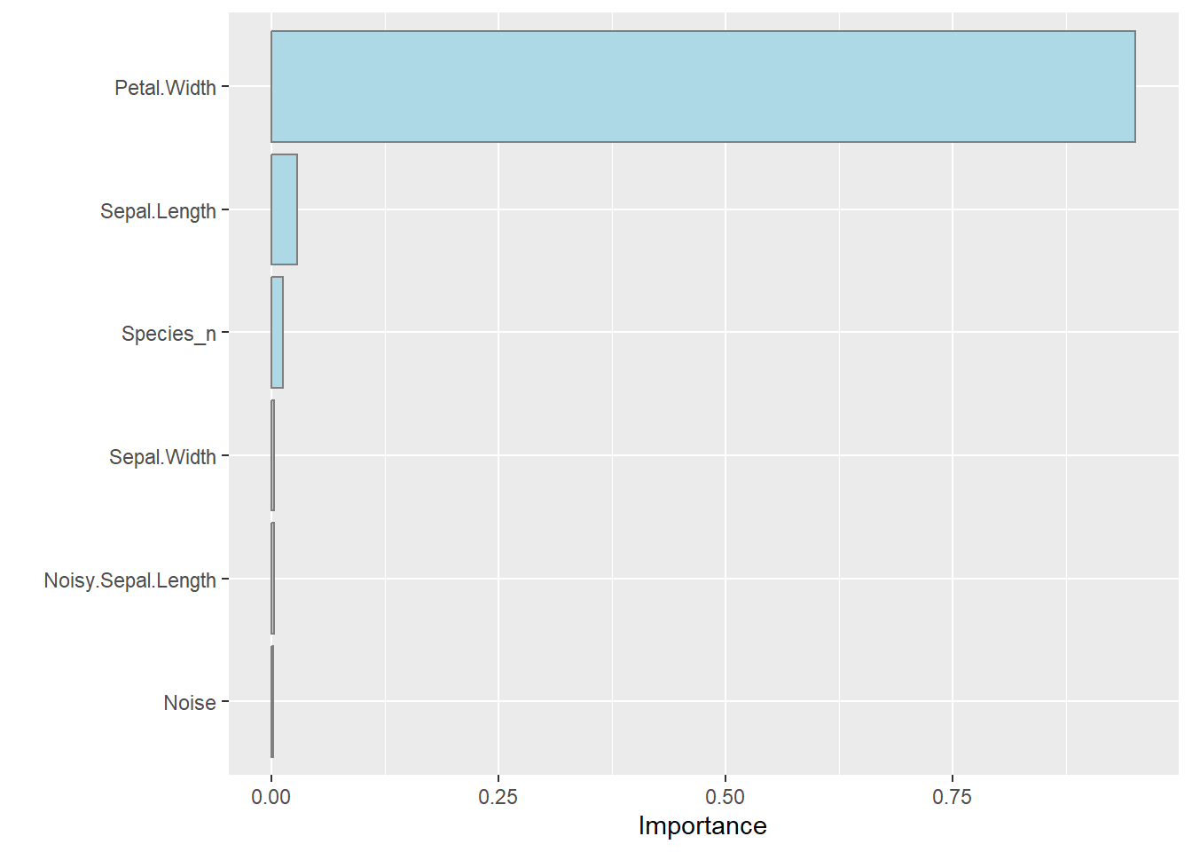
It is interesting that the xgboost importance is different to the random forest and linear models. The model is good as shown in the scatterplot below:
# then do a quick check on the output
pred.iris_xgb <- predict(model_reg_xgboost, iris_reg_test)
bind_cols(iris_reg_test$Petal.Length, pred.iris_xgb) %>%
  rename(actual = ...1, pred = .pred) %>%
  ggplot(aes(actual, pred)) +
  geom_point() +
  ggpubr::stat_regline_equation(aes(label =  paste(after_stat(eq.label),
                                                   after_stat(adj.rr.label), sep = "~~~~"))) +
  geom_smooth(method = "lm") +
  geom_abline(slope = 1, intercept = 0) +
  labs(title = "The xgboost model is good a predicting Petal.Length",
       subtitle = "This plot shows performance on unseen data",
       x = "Actual Petal Length", y = "Model estimate of Petal Length")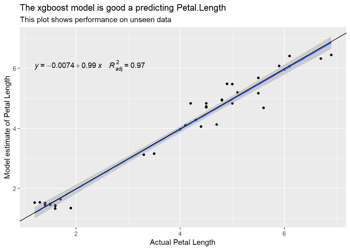
However, the set of rules that generates the result is 67626 characters long and utterly impenetrable! Have a look at the spreadsheet I’ve generated if you’re interested. because it’s so long it is too large to be evaluated in Excel. To shoehorn this model into Excel I have hacked some logic to treat it as it if was 15 different trees, then adapted the summary to add rather than average the trees. It’s all in the code if anyone really wants to see how I managed it.
Below I’ve plotted modelled and actual outputs for each of the models using the test dataset.
# creating ggplot object for visualization

iris_reg_test %>%
  select(Petal.Length, Species) %>%
  bind_cols(predict(model_reg_lm, iris_reg_test) %>%
              enframe(name = NULL, value = "full_lm")
            ) %>%
  bind_cols(predict(model_reg_lm_simplified, iris_reg_test) %>%
              enframe(name = NULL, value = "simplified_lm")
            ) %>%
  bind_cols(pred.iris_rf$predictions) %>%
  rename(Random_Forest = ...5) %>%
  bind_cols(pred.iris_xgb) %>%
  rename(XGBoost = .pred) %>%
  pivot_longer(-c(Petal.Length, Species), names_to = "model", values_to = "estimate") %>%
  ggplot(aes(Petal.Length, estimate)) +
  geom_point(aes(colour = Species)) +
  ggpubr::stat_regline_equation(aes(label =  paste(after_stat(eq.label),
                                                   after_stat(adj.rr.label), sep = "~~~~")), size = 4) +
  geom_smooth(method = "lm") +
  facet_wrap( ~ model) +
  labs(title = "All the regession models do a good job of predicting Petal Length",
       subtitle = "This plot is based on the test dataset",
       x = "True Petal Length",
       y = "Modelled Petal Length")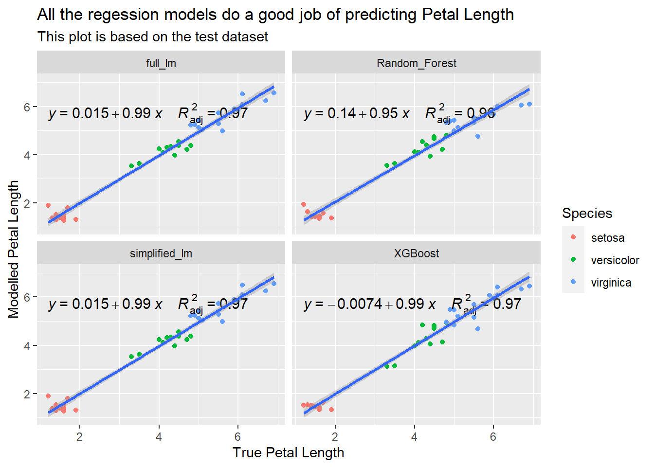
All the models do a good job of predicting Petal.Length. In this case, I would say that the linear models would be the most attractive choice given their accuracy and simplicity but I haven’t tried to tune the more complex ML models, and the problem domain is well suited to linear models, not all datasets have such clean relationships. If you look back at those scatter-plots I made right at the start when exploring the iris dataset, Petal.Length was very strongly correlated to Petal.Width… In reality, if I needed a model to predict Petal.Length I probably wouldn’t have access to Petal.Width!
Let’s look at the importance of the explanatory variables from the perspective of each of the regression models we’ve built:
vip::vi(model_reg_lm) %>% mutate(Model = "full lm", .before = 1) %>%
  bind_rows(
    vip::vi(model_reg_lm_simplified) %>% mutate(Model = "simplified lm", .before = 1)
  ) %>%
  bind_rows(
    vip::vi(model_reg_rf) %>% mutate(Model = "Random Forest", .before = 1)
  ) %>%
  bind_rows(
    vip::vi(model_reg_xgboost) %>% mutate(Model = "XGBoost", .before = 1)
  ) %>%
  mutate(Sign = coalesce(Sign, "Undefined")) %>%
  mutate(Importance = ifelse(Sign == "NEG", 0-Importance, Importance)) %>%
  ggplot(aes(x = Variable, y = Importance, fill = Sign)) +
  geom_col() +
  coord_flip() +
  facet_wrap( ~ Model, scales = "free_x") +
  labs(title = "This plot shows what each model relied on to estimate Petal Length",
       subtitle = "The linear model models work quite differently to the tree-based ones")
At first inspection it may appear surprising that each model attributes different importance to each explanatory variable. However, I’ll make three observations:
Three of the models rely heavily on Species. The Linear models in the above example are structured slightly differently to the tree-based ones. The tree-based ones use Species via Species_n while the linear models represent Species using Speciesvirginica, Speciesversicolor (and implicitly, Speciessetosa through the offset)
Linear models are fitted quite differently to the tree-based ones. Unless explicitly asked to do so (e.g. by using interactions), linear models build relationships (regress) on relationships across the entire space of how the Petal.Length varies with explanatory variables. The tree-based techniques chop the space into smaller and smaller internally consistent chunks as a function of some notion of impurity). This allows tree-based techniques to handle relationships that only hold in part of the space. They can handle non-linearities in the same way.
With the above two points in mind, I’m most surprised at how well xgboost managed to perform while apparently mostly relying on Petal.Width
So far I have:
Fitted a few models.
Translated these models into if() logic that Excel can execute
… I still need to:
Add some columns that summarise the ‘best’ model (remember random forests are made up of many decision trees, each tree offers a suggestion of the answer we’re after)
Package the data and the models (as formula) into something that can be loaded into Excel
Building the best output (and some kind of indicator on the confidence of that answer) is slightly different for classification and regression. The table below summarises the key differences.
| Statistic | Classification | Regression |
|---|---|---|
| Best model | Modal (most common) result from all trees = INDEX(L2:BI2, MODE(MATCH(L2:BI2, L2:BI2, 0 ))) |
Mean (average) result from all trees = AVERAGE(M2:BJ2) |
| Confidence in Best model | Percentage of all models agreeing with the best model =COUNTIF(L2:BI2, H2) / COUNTA(L2:BI2) |
normalised variance of all tree estimates = 1-SQRT(VAR(M2:BJ2, I2)) / AVERAGE(M2:BJ2) |
| Accuracy | Logical ( True if the best model correctly classified the example = (modelled = actual) |
percentage error = (modelled - actual) / actual |
#' @title add.formula
#'
#' @description
#' decorates a column in a dataframe with 'formula'
#' doingf this makes excelk evaluate the contents rather than just
#' treating them as a string and presenting the formaula rather than its result
#' thanks here to: https://stackoverflow.com/questions/45579287/r-assign-class-using-mutate
add.formula <- function(x) {class(x) <- c(class(x), "formula"); x}

#' @title add.formula
#'
#' @description
#' things function returns the letter of a column index by x in Excel format
#' Excel has a col::row reference system with letters::numbers
#' the letters (columns) starft at 'A',  continue until 'Z' then 'AA'-'ZZ'
#'
#' @param x the columns number (starting from 1 -> 'A')
#'
#' @return string containing the Excel letter-based column reference
#'
get_excel_letter <- function(x) {
  paste0(LETTERS[((x-1) %/% 26)], LETTERS[1+((x-1) %% 26)])
}


#' @title augment_df_with_rules
#'
#' @description
#' This function takes a list of models (e.g. a LM, or many decision trees)
#' and transforms them so that they act on the "in_df" as per Excel
#' @param models a 1D df containing one row per model
#' @param in_df The dataframe upon which the model is to be used
#' @param target The names of the target variable (must be in the in_df)
#' @param method classification or regression (this affects how trees are agregated)
#'
#' @return a character string with the "html" class and "html" attribute
#'
#' @export
#'
#' @examples
#' asHTML("<p>This is a paragraph</p>")
#'
augment_df_with_rules <- function(models, in_df, target = NA, method = "classification") {
  # were' going to insert a few stats cols after the input data so
  # the start of the trees will be at this column:
  nstats <- 3 # I'm adding 3 extra columns (best, confidence and match)
  index_of_target <- which(names(in_df) == target)
  if(length(index_of_target)==0) {
    stop("augment_df_with_rules: target (", target, ") could not be found")
  }
  trg_col <- get_excel_letter(index_of_target) # this is where thhe target is in the dataset
  trg_ref_col <- get_excel_letter(ncol(in_df)+1) # this the  target copied into the end of the dataset
  mod_col <- get_excel_letter(ncol(in_df)+2) # this is the col of the best model
  first_model_col <- get_excel_letter(ncol(in_df)+nstats+2) # start of options for model output
  last_model_col  <- get_excel_letter(ncol(models)+ncol(in_df)+nstats+1) # end of options for model output

  result_df <- in_df %>%
    as_tibble() %>%
    bind_cols(models)

  if(method == "classification") {
    result_df <- result_df %>%
      mutate(tree_target = glue::glue("={trg_col}[ROW_NUM]"), .before = tree_1) %>%
      mutate(tree_best = glue::glue("=INDEX({first_model_col}[ROW_NUM]:{last_model_col}[ROW_NUM], MODE(MATCH({first_model_col}[ROW_NUM]:{last_model_col}[ROW_NUM], {first_model_col}[ROW_NUM]:{last_model_col}[ROW_NUM], 0 )))"), .before = tree_1) %>%
      mutate(tree_confidence = glue::glue("=COUNTIF({first_model_col}[ROW_NUM]:{last_model_col}[ROW_NUM], {trg_ref_col}[ROW_NUM]) / COUNTA({first_model_col}[ROW_NUM]:{last_model_col}[ROW_NUM])"), .before = tree_1) %>%
      mutate(tree_match = glue::glue("={mod_col}[ROW_NUM]={trg_ref_col}[ROW_NUM]"), .before = tree_1)
  } else {
    result_df <- result_df %>%
      mutate(tree_target = glue::glue("={trg_col}[ROW_NUM]"), .before = tree_1) %>%
      mutate(tree_best = glue::glue("=AVERAGE({first_model_col}[ROW_NUM]:{last_model_col}[ROW_NUM])"), .before = tree_1) %>%
      mutate(tree_confidence = glue::glue("=1-SQRT(VAR({first_model_col}[ROW_NUM]:{last_model_col}[ROW_NUM], {trg_ref_col}[ROW_NUM])) / AVERAGE({first_model_col}[ROW_NUM]:{last_model_col}[ROW_NUM])"), .before = tree_1) %>%
      mutate(tree_match = glue::glue("=({mod_col}[ROW_NUM]-{trg_ref_col}[ROW_NUM])/{trg_ref_col}[ROW_NUM]"), .before = tree_1)
  }

  result_df <- result_df %>%
    mutate(row_num = as.character(row_number()+1)) %>% # +1 because in Excel there's a title in row 1
    # fold in the actual row number instead of that place holder "ROW_NUM"
    mutate_at(vars(starts_with("tree")), list(~ str_replace_all(., "\\[ROW_NUM\\]", row_num))) %>%
    # decorate the calculation columns as formula so Excel will show the results rather than the equations
    mutate_at(vars(starts_with("tree")), add.formula) %>%
    select(-row_num)

  return(result_df)
}Let’s use the functions to build the final data-frames that contain everything we need to write to Excel…
#| turn the tidypredict_sql for all the trees into a tidy dataframe

#| random forest classification in Excel format ----
trees_df_iris_rf_clas <- tidypredict::tidypredict_sql(model_clas_rf, dbplyr::simulate_dbi()) %>%
  tibble::enframe(name = NULL, value = "instruction") %>%
  mutate(instruction = unlist(instruction))

randforest_clas <- sql_to_excel(trees_df = trees_df_iris_rf_clas, input_df = iris_n_noise)
model_output_clas <- augment_df_with_rules(models = randforest_clas,
                                           in_df = iris_n_noise,
                                           target = "Species",
                                           method = "classification")

# this emulates LM in Excel format ----
trees_df_lm <- tidypredict::tidypredict_fit(model_reg_lm)[2] %>% as.character() %>%
  tibble::enframe(name = NULL, value = "instruction") %>%
  mutate(instruction = unlist(instruction)) %>%
  mutate(instruction = as.character(instruction))
# make Excel-friendly
lm_excel <- fit_to_excel(trees_df = trees_df_lm, input_df = iris_n_noise)
model_output_lm <- augment_df_with_rules(models = lm_excel,
                                         in_df = iris_n_noise,
                                         target = "Petal.Length",
                                         method = "regession")

# random forest regression in Excel format ----
# get the rules
trees_df_iris_rf_reg <- tidypredict::tidypredict_sql(model_reg_rf, dbplyr::simulate_dbi()) %>%
  tibble::enframe(name = NULL, value = "instruction") %>%
  mutate(instruction = unlist(instruction))

# convert the rules to Excel format
randforest_reg <- sql_to_excel(trees_df = trees_df_iris_rf_reg, input_df = iris_n_noise_reg)
dim(randforest_reg) #one row but many columns (one per tree)
[1] 1 50model_output_iris_reg <- augment_df_with_rules(models = randforest_reg,
in_df = iris_n_noise_reg,
target = "Petal.Length",
method = "regression")
# xgboost regression in Excel format ----
# get the rules
raw_xbg_rules <- tidypredict::tidypredict_sql(model_reg_xgboost, dbplyr::simulate_dbi()) %>%
unlist() %>%
as.character()
# xgboost adds a constant at te end of it's logic
# and my sql_to_excel function doesn't handle it well *it nests it at an unused ent of an if statement_
# Im hacking now to make this work... I'll ... erm...
# 1) separate if from the rest of the formula
# handle the first part as normal(ish)
# and add it as a lonesome rule at the end
last_part <- sub(".+\\s([\\+\\-]\\s*[0-9\\.]+)$", "\\1", raw_xbg_rules)
first_part <- str_replace(raw_xbg_rules, paste0("\\", last_part), "")
trees_df_iris_xgboost_reg <- first_part %>%
tibble::enframe(name = NULL, value = "instruction") %>%
mutate(instruction = unlist(instruction)) %>%
# extra steps needed to tidy the format of the xgboost tidypredict_sql
# we dont need any 0.0 + lines
mutate(instruction = str_remove_all(instruction, "0.0 \\+ ")) %>%
# remove all leading brackets
mutate(instruction = str_remove(instruction, "^\\(+")) %>%
# parts of the tree are additive, so te tree is *very* long (and exceeds the token limit in LibreOffice)
# so I've decided to split the additive components into separate rows
# as if the are their own separate trees
# NOTE: in random forests we AVERAGE the trees, in xgboost we must ADD the trees
separate_rows(instruction, sep = "\\+ CASE") %>%
# the first CASE is still here..., I'll delete it..
mutate(instruction = str_remove(instruction, "CASE")) %>%
# we need to put the "CASE" back!
# I used to split the single rule (on that specific "+") into many separate ones
# but now need it back for the logic to make sense
mutate(instruction = paste0("CASE", instruction))
# convert the rules to Excel format
xgboost_reg <- sql_to_excel(trees_df = trees_df_iris_xgboost_reg, input_df = iris_reg_train) %>%
pivot_longer(cols = everything(), names_to = "tree", values_to = "instruction") %>%
# remove the last bracket (dont know why ther's an extra one
# maybe there's a linefeed at the end of each additive part of xgboost)
mutate(len_before = str_length(instruction), .before = tree) %>%
mutate(instruction = str_remove(instruction, "\\)$")) %>%
mutate(len_after = str_length(instruction), .before = tree) %>%
select(-c(len_before, len_after)) %>%
bind_rows(
paste0("= ", last_part) %>%
enframe(name = NULL, value = "instruction") %>%
mutate(tree = "tree_const", .before = 1)
) %>%
pivot_wider(names_from = "tree", values_from = "instruction")
model_output_iris_xgboost_reg <- augment_df_with_rules(models = xgboost_reg,
in_df = iris_n_noise_reg,
target = "Petal.Length",
method = "regression")The functions changes logic that looks like this:
trees_df_iris_rf_clas[1,]# A tibble: 1 × 1
instruction
<chr>
1 "CASE\nWHEN (`Petal.Length` < 3.1 AND `Sepal.Width` >= 3.25) THEN 'setosa'\nW…into logic that looks like this:
model_output_clas[1,"tree_1"]# A tibble: 1 × 1
tree_1
<chr>
1 "=if(and(C2<3.1,B2>=3.25),\"setosa\",if(and(C2<2.45,C2<4.95,B2<3.25),\"setosa…The resultant dataframe has 150 rows (one per example of iris), and 61 columns. The columns are best summarised as three blocks:
The first block (of 7 columns) holds the iris data itself as described right at the outset.
The second block (of 4 columns) holds some summaries (which I’ll expand on in a moment)
The third block (of 50 columns) holds 50 formulae that encapsulate the 50 trees generated within the random forest model.
I hope blocks 1 and 3 have been expo’d already throughput this post. The middle block (placed in the middle as they join the input data to all those individual trees by summarising the results) was described at the start of this section but is expanded below for clarity:
Target variable: I have chosen to carry the target variable (Species for classification and Petal.Length for regression) into a new column for clarity. Having it duplicated may be a little redundant but I think it makes the spreadsheets easier to read. For example, the first target in the regression models is =C2 (C is the column holding Petal.Length and the first equation is in row 2 as the column titles are in the first row.
Model output: The model output is some kind of aggregate of the outputs of the individual trees. For classification, the model output for the first example is the most frequently suggested classification of all 50 models. The formula is: =INDEX(L2:BI2, MODE(MATCH(L2:BI2, L2:BI2, 0 ))). For regression it is simply the average estimate from all the models (trees). The formula for the best model is: =AVERAGE(M2:BJ2)
Model Confidence: I’ve chosen to use the following calculations to represent the confidence in the model outputs. For classification the column contains: =COUNTIF(L2:BI2, H2) / COUNTA(L2:BI2) and for regression it is: =1-SQRT(VAR(M2:BJ2, I2)) / AVERAGE(M2:BJ2) .
Model Match: For classification this is some test of equality: =I2=H2. For regression I’ve used a percentage error metric: =(J2-I2)/I2
Each cell in Spreadsheet has a limited number of characters. At the time of writing this is 32,767 characters in Excel. In libreOffice Calc it’s even larger but shrinks to many fewer ‘tokens’. Lets have a look at how many characters are in each decision tree:
  # the trees can be quite long as every condition is defined as "IF",
  # most of the conditions for the next case are really just "ELSE"
  # but this way makes things much easier to read as a human
  # Excel's nested if(this, that, if(other...)) quickly become impenetrable
  randforest_clas %>%
    pivot_longer(cols = everything(), names_to = "tree_id", values_to = "tree_content") %>%
    mutate(model = "Classification", .before = tree_id) %>%
    mutate(tree_length = str_length(tree_content), .after = tree_id) %>%
    bind_rows(
      randforest_reg %>%
        pivot_longer(cols = everything(), names_to = "tree_id", values_to = "tree_content") %>%
        mutate(model = "Regression", .before = tree_id) %>%
        mutate(tree_length = str_length(tree_content), .after = tree_id)
    ) %>%
    group_by(model) %>%
    arrange(desc(tree_length)) %>%
    mutate(row_num = row_number()) %>%
    ungroup() %>%
    ggplot(aes(x = row_num, y = tree_length, colour = model)) +
    geom_point() +
    labs(title = "Regression trees are considerably more complex than ones for classification",
         subtitle = "Each forest as 50 trees. Some trees are more complicated than others",
         x = "", y = "Number of characters in the rule that defines the tree") +
    facet_wrap( ~ model)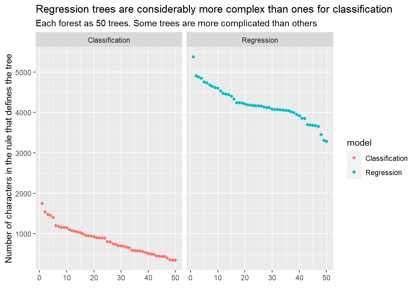
If I had not shrunk the number of characters by removing whitespace and limiting the number of significant figures, the random forest rules can exceed what can be represented in LibreOffice Calc. The xgboost model was too large to run in LibreOffice but with a little manipulation (to separate each of the 15 additive components into separate cells), even xgboost can be accommodated.
There are packages that make it easy to create an Excel workbook with multiple tabs, one for each example I created above. I’m using {openxlsx} and writing each data-frame I created previously into a separate tab. The code is folded below.
# Creating Excel workbook..
output_wb <- openxlsx::createWorkbook(creator = "Leo Kiernan", subject = paste0("Ranger random forest model ", lubridate::now()))
openxlsx::addWorksheet(output_wb, "README", tabColour = "blue")
openxlsx::addWorksheet(output_wb, "RF_classification", tabColour = "orange")
openxlsx::addWorksheet(output_wb, "LM_regression", tabColour = "green")
openxlsx::addWorksheet(output_wb, "RF_regression", tabColour = "red")
openxlsx::addWorksheet(output_wb, "XGB_regression", tabColour = "purple")
openxlsx::addWorksheet(output_wb, "RF_classificationRules", tabColour = "orange")
openxlsx::addWorksheet(output_wb, "LM_regressionRules", tabColour = "green")
openxlsx::addWorksheet(output_wb, "RF_regressionRules", tabColour = "red")
openxlsx::addWorksheet(output_wb, "XGB_regressionRules", tabColour = "purple")

# Populating Excel workbook...
# first the README tab
tribble(
  ~from, ~tab, ~info,
  "LAK", "README", "This sheet",
  "LAK", "RF_classification", "An example of a classification of Iris Species using random forest",
  "LAK", "LM_regression", "An example of a regression to predict Petal Length using a linear model",
  "LAK", "RF_regression", "An example of predicting Petal Length using random forest regression",
    "LAK", "XGB_regression", "An example of predicting Petal Length using a xgboost regression",
  "LAK", "RF_classificationRules", "One row per tree in the classification random forest.  Easy-to-read SQL logic format",
  "LAK", "LM_regressionRules", "The internal equations in the linear model in an easy-to-read format",
  "LAK", "RF_regressionRules", "One row per tree in the regression random forest.  Easy-to-read SQL logic format",
  "LAK", "XGB_regressionRules", "The single HUGE xgboost rule.  Easy-to-read SQL logic format"
) %>%
  mutate(Date = lubridate::now(), .before = 1) %>%
  openxlsx::writeDataTable( wb = output_wb,
                            sheet = "README",
                            x = .,
                            startCol = 1,
                            startRow = 1,
                            tableStyle = "TableStyleLight9",
                            tableName = "README")

# classification tree ----
model_output_clas %>%
  openxlsx::writeDataTable( wb = output_wb,
                            sheet = "RF_classification",
                            x = .,
                            startCol = 1,
                            startRow = 1,
                            tableStyle = "TableStyleLight9",
                            tableName = "RF_classification")

trees_df_iris_rf_clas  %>%
  openxlsx::writeDataTable( wb = output_wb,
                            sheet = "RF_classificationRules",
                            x = .,
                            startCol = 1,
                            startRow = 1,
                            tableStyle = "TableStyleLight9",
                            tableName = "RF_classificationRules")


# lm ----
model_output_lm %>%
  openxlsx::writeDataTable( wb = output_wb,
                            sheet = "LM_regression",
                            x = .,
                            startCol = 1,
                            startRow = 1,
                            tableStyle = "TableStyleLight9",
                            tableName = "LM_regression")

trees_df_lm  %>%
  openxlsx::writeDataTable( wb = output_wb,
                            sheet = "LM_regressionRules",
                            x = .,
                            startCol = 1,
                            startRow = 1,
                            tableStyle = "TableStyleLight9",
                            tableName = "LM_regressionRules")

# RF regression tree ----
model_output_iris_reg %>%
  openxlsx::writeDataTable( wb = output_wb,
                            sheet = "RF_regression",
                            x = .,
                            startCol = 1,
                            startRow = 1,
                            tableStyle = "TableStyleLight9",
                            tableName = "RF_regression")
trees_df_iris_rf_reg  %>%
  openxlsx::writeDataTable( wb = output_wb,
                            sheet = "RF_regressionRules",
                            x = .,
                            startCol = 1,
                            startRow = 1,
                            tableStyle = "TableStyleLight9",
                            tableName = "RF_regressionRules")

# xgboost tree ----
model_output_iris_xgboost_reg %>%
  # one final hack to get xgboost working (it's a sum of components, not an average of trees)
  mutate(tree_best = str_replace(tree_best, "AVERAGE\\(", "SUM\\(")) %>%
  # we've edited the tree_best column so we need to re-assert it is a formula
  mutate_at(vars(starts_with("tree")), add.formula) %>%
  openxlsx::writeDataTable( wb = output_wb,
                            sheet = "XGB_regression",
                            x = .,
                            startCol = 1,
                            startRow = 1,
                            tableStyle = "TableStyleLight9",
                            tableName = "XGB_regression")
# xgboost is "different". I'll show the raw output
tidypredict::tidypredict_sql(model_reg_xgboost, dbplyr::simulate_dbi()) %>%
  tibble::enframe(name = NULL, value = "instruction") %>%
  mutate(instruction = unlist(instruction))  %>%
  openxlsx::writeDataTable( wb = output_wb,
                            sheet = "XGB_regressionRules",
                            x = .,
                            startCol = 1,
                            startRow = 1,
                            tableStyle = "TableStyleLight9",
                            tableName = "XGB_regressionRules")
Warning in wb$writeData(df = x, colNames = TRUE, sheet = sheet, startRow = startRow, : S NULL)) AND (`S ... 29585
END) + 0.5 is truncated.
Number of characters exeed the limit of 32767.# Save Excel workbook...
openxlsx::saveWorkbook(wb = output_wb,
file = here::here(stringr::str_c("posts/ML_in_excel/ml_in_excel.xlsx")),
overwrite = T)In this blog I have shown how Machine Learning models can be delivered in Excel. I have fitted the models outside Excel (in R), explored their performance and what things they find important, and then then converted the model equations into excel formulae. I’ve demonstrated how to generate Excel formulae for linear models, decision trees, random forests and xgboost. However, at the time of writing, the logic I’ve written in this post would work for a whole range of other models: Linear Regression - lm(), Generalized Linear model - glm(), Random Forest models - randomForest::randomForest(), Random Forest models, via ranger - ranger::ranger() , MARS models - earth::earth() , XGBoost models - xgboost::xgb.Booster.complete(), Cubist models - Cubist::cubist() and Tree models, via partykit - partykit::ctree().
I’ve not optimised the models, but I have added links that describe how such models could be optimised. The optimised models are the same shape as the ones I’ve built, hence they would be exported into Excel in exactly the same way. Also, I chose a simple dataset on which to train the models which may have allowed the linear models to shine for it’s simplicity, interperability and accuracy. But in general random forests and xgboost are extremely popular and effective methods for modelling data.
I’ll end on a ridiculously optimistic thought by returning to that statistic provided by Microsoft:
“hundreds of millions of people use Excel”
“and many of them use it to build themselves sophisticated tools that go far beyond the original capabilities of a spreadsheet.”…
Imagine…
If one-in-a-thousand Excel users would benefit from access to machine Learning in Excel, maybe this post could be of benefit to hundreds of thousands of people.
I hope the handful of people that have actually read this far have found it interesting and useful in some way ;-P
Itch scratched.
Since I first published this post I’ve had some valuable feedback (thanks @nabsiddiqui@h-net.social) and pointers to extra resources on this subject. Here’s some further reading:
All the code used in this and other posts are available here.
At the outset of this post I caveated my promise to “end up with something that anyone with access to a spreadsheet can use for regression or classification tasks” with small-print “just so long as the datasets are not too big or the decision space too complex”. I’d like to take a little time to unpack that statement here. Spreadsheets are extremely versatile and powerful but are not the most efficient ways to handle large amounts of data and are limited in the complexity of models that they can hold. IMHO there are four main attributes of spreadsheets that one should be aware of to be able to consider whether they’re the right place for certain tasks:
Some big limits matter in this context:
The number of rows (often analogous to the number of records in a data-frame).
The number of columns (number of fields and calculations on the data-frame).
The number of characters you can enter into any individual cell (analogous to the complexity of any calculation you may wish to perform).
I’ve just checked the limits for Excel (see here) and I am honestly surprised how large these limits are nowadays, so perhaps the hard-limits would not be reached for most practical purposes, but the .xlsx file sizes for any models pushing close to these limits would be enormous! Note: Sure, you can write scripts in spreadsheets to undertaken tasks that would be overly cumbersome in the cells, but this is just taking one-step out of spreadsheets into the world of code and can be a sign that perhaps the spreadsheets are reaching their limit and alternative solutions could and should be considered.
In this post I’ve generated random forests of 50 decision trees. Each tree is implemented in a column in the spreadsheet. Often random forests have thousands of trees. Trees can be quite big, regression trees are often larger than classification trees. The logic for big trees takes a lot of IF() functions in Excel and much of my challenge in this post has been to shrink the decision tree logic such that meaningfully complex trees can fit in each cell in Excel.
Reactivity is the spreadsheets ability to present the answers as soon as data changes. For example, if you average the values in a range, when the data in the range changes, the averages changes automatically, the average reacts to the change of inputs. This feature is a real advantage in relatively simple use-cases but it works even if there’s a long chain of calculations between the input and output. In large spreadsheets this reactivity soon turns from a blessing to a curse. Spreadsheets can have the auto-recalculation temporarily disable to improve performance but it’s really just a work-around.
Spreadsheets hold data and calculations. You can use power-query to push some of the calculations upstream into databases etc. Separating data from business logic, from reporting becomes more and more important as the scale of the task increases. Large-scale analytic solutions almost always allow logical separation of data from algorithms and visualisations or reports. This separation has real value (see reusabilty limits below).
Disentangling data from algorithms also significantly improves auditability. Anyone who has every found a rogue calculation change part-way down a long (and supposedly consistent) set of calculations will attest to the uncomfortable feeling it brings. The veracity of large spreadsheets is almost impossible to verify.
Spreadsheets do not promote modularisation or reusability. Linked spreadsheets are an option to allow modularisation, but there’s a massive overhead that comes with such approaches. If you do not carefully honour that overhead the entire chain of spreadsheets becomes untrustworthy, unauditable and unsustainable. In my experience linked spreadsheets are a sign of creeping growth in analytic or reporting capability that cries out for re-factoring and reassessment.
or other spreadsheets such as LibreOffice Calc↩︎
See the discussion section for mode on these points↩︎
with the usual disclaimers around ‘The postings on this site are my own and do not necessarily reflect the views of [Employer].’ etc.↩︎
In general you may not know up-front what packages you need. packages come into play ask you move through the various phases of load-explore–model-summarise-export. The list of packages has got longer as I’ve attempted more and more steps in this post. I could’ve loaded each library at the point I need them in the code (or references them using {package}::{function} as per the stringi example in one of my functions) but I’ve chosen to load them all up-front just as a convention.↩︎
The dataset is relatively simple to feed into a classifier because the classes (Species) are ‘balanced’ (which just means there’s the same number of examples in each class). The ML community have developed plenty of ways that to handle unbalanced classes but anyone undertaking ML classification must consider this when constructing any ML solution.↩︎
like random-forests, neural-networks and boosted trees etc↩︎
complexity penalty functions, regularisation bootstrapping, (n-fold) cross validation are just a few↩︎
The training data is often further split into training and validation. Where the former is used to defined the parameters of the model and the latter is held-out to check how the model might perform on genuinely new data unavailable at the time when the model was trained. The validation sets are used to stop the model “over fitting” (memorising) the input/output relationships of the training data and having little or no generalisability when presented with new data. Think of a student revising for a maths exam… They could learn the answer for some question (by rote) or the way in which the answer can be calculated. When we ask a ML system to learn something from data, more-often than not, we’d like to capture some underlying relationship rather than be some look-up table.↩︎
In the implementation of random forests I’m using, the bit that translates each tree into SQL doesn’t handle categorical variables very elegantly. It translates them into counting numbers, so the iris class becomes 1, 2 &3. not a huge issue, but I would’ve rather it have captured the categorical input data as elegantly as the LM clearly does (read on)↩︎